

Problems 285
(c) Calculate the values for the same periods, but using a mean
recurrence of 132 years and a standard deviation of 105
years, which correspond to the full Pallett Creek earthquake
series. Explain how and why the results change.
C-9. Use the routine from C-8 to estimate the Poisson and Gaussian
conditional probabilities of a major earthquake in the New
Madrid seismic zone in the next 20 years, assuming that the past
one occurred in 1812. Assume that major earthquakes have:
(a) a mean recurrence time of 500 years with standard
deviation 100 years.
(b) a mean recurrence time of 750 years with standard
deviation 250 years.
(c) a mean recurrence time of 1000 years with standard
deviation 500 years.
C-10. Write a subroutine (or set up a spreadsheet) to compute the
mean and standard deviation of series of numbers.
C-11. By combining the results from C-8 and C-10:
(a) Find the mean and standard deviation of recurrence intervals for the series of Parkfield earthquakes that occurred
in the years 1857, 1881, 1901, 1922, 1934, and 1966.
Compute Poisson and Gaussian conditional probabilities
starting in 1985 for an earthquake in the eight-year interval until 1993.
(b) Do the same calculation if the 1934 earthquake had
occurred in 1944, as implicitly assumed when the prediction discussed in Section 1.2.5 was made. How do the
values change and why?
(c) The awaited earthquake may or may not have occurred
by the time you do this problem. In either event, assume
that it has not occurred by 2010, and find the mean and
standard deviation of the recurrence times from the dates
in (a), also including the interval 1966–2010. Calculate
the Poisson and Gaussian conditional probabilities that
the earthquake will occur in eight years from 2010.
(d) Do the same assuming the earthquake has not occurred
by 2020.
(e) Compare the results of (a), (c), and (d) and explain the
differences.
(b) Use this routine to find the directions of the P and T axes for
the focal mechanisms in problem 2. Compare your results to
those obtained in C-2.
C-5. Write subroutines to generate the amplitude radiation patterns
for Love and Rayleigh waves. Use these, with values of the
excitation functions
P L = −2.75, Q L = − 0.34, and S R = 4.0, P R = 2.7, Q R = −1.6
to replicate the examples of Fig. 4.3-12.
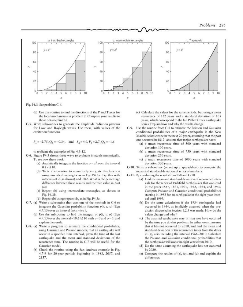
C-6. Figure P4.3 shows three ways to evaluate integrals numerically.
To see how these work:
(a) Analytically integrate the function y = x 2 over the interval
0 ≤ x ≤ 10.
(b) Write a subroutine to numerically integrate this function
using inscribed rectangles as in Fig. P4.3a. Try this with
intervals of 2 (as shown) and 0.02. What is the percentage
difference between these results and the true value in part
(a)?
(c) Repeat (b) using intermediate rectangles, as shown in
Fig. P4.3b.
(d) Repeat (b) using trapezoids, as in Fig. P4.3c.
C-7. (a) Write a subroutine that uses one of the methods in C-6 to
integrate the Gaussian probability function p(t, τ, σ) (Eqn
4.7.13) over an interval from −t to t.
(b) Use the subroutine to find the integral of p(t, τ, σ ) (Eqn
4.7.13) over the interval −10 ≤ t ≤ 10 with τ = 0 and σ = 5, and
explain the result.
C-8. (a) Write a program to estimate the conditional probability,
using Gaussian and Poisson models, that an earthquake will
occur in a specified time interval, given the time of the last
earthquake and the mean and standard deviations of the
recurrence time. The routine in C-7 will be useful for the
Gaussian model.
(b) Check the routine using the San Andreas example in Fig.
4.7-9 for 20-year periods beginning in 1983, 2057, and
2157.
Fig. P4.3 See problem C-6.
y
100
80
60
40
20
0
10
y = x
2
a. Inscribed rectangles
0 1 2 3 4 5 6 7 8 9
x
y
100
80
60
40
20
0
10
y = x
2
b. Intermediate rectangles
0 1 2 3 4 5 6 7 8 9
x
y
100
80
60
40
20
0
10
y = x
2
c. Trapezoids
0 1 2 3 4 5 6 7 8 9
x
(c) Calculate the values for the same periods, but using a mean
recurrence of 132 years and a standard deviation of 105
years, which correspond to the full Pallett Creek earthquake
series. Explain how and why the results change.
C-9. Use the routine from C-8 to estimate the Poisson and Gaussian
conditional probabilities of a major earthquake in the New
Madrid seismic zone in the next 20 years, assuming that the past
one occurred in 1812. Assume that major earthquakes have:
(a) a mean recurrence time of 500 years with standard
deviation 100 years.
(b) a mean recurrence time of 750 years with standard
deviation 250 years.
(c) a mean recurrence time of 1000 years with standard
deviation 500 years.
C-10. Write a subroutine (or set up a spreadsheet) to compute the
mean and standard deviation of series of numbers.
C-11. By combining the results from C-8 and C-10:
(a) Find the mean and standard deviation of recurrence intervals for the series of Parkfield earthquakes that occurred
in the years 1857, 1881, 1901, 1922, 1934, and 1966.
Compute Poisson and Gaussian conditional probabilities
starting in 1985 for an earthquake in the eight-year interval until 1993.
(b) Do the same calculation if the 1934 earthquake had
occurred in 1944, as implicitly assumed when the prediction discussed in Section 1.2.5 was made. How do the
values change and why?
(c) The awaited earthquake may or may not have occurred
by the time you do this problem. In either event, assume
that it has not occurred by 2010, and find the mean and
standard deviation of the recurrence times from the dates
in (a), also including the interval 1966–2010. Calculate
the Poisson and Gaussian conditional probabilities that
the earthquake will occur in eight years from 2010.
(d) Do the same assuming the earthquake has not occurred
by 2020.
(e) Compare the results of (a), (c), and (d) and explain the
differences.
(b) Use this routine to find the directions of the P and T axes for
the focal mechanisms in problem 2. Compare your results to
those obtained in C-2.
C-5. Write subroutines to generate the amplitude radiation patterns
for Love and Rayleigh waves. Use these, with values of the
excitation functions
P L = −2.75, Q L = − 0.34, and S R = 4.0, P R = 2.7, Q R = −1.6
to replicate the examples of Fig. 4.3-12.
C-6. Figure P4.3 shows three ways to evaluate integrals numerically.
To see how these work:
(a) Analytically integrate the function y = x 2 over the interval
0 ≤ x ≤ 10.
(b) Write a subroutine to numerically integrate this function
using inscribed rectangles as in Fig. P4.3a. Try this with
intervals of 2 (as shown) and 0.02. What is the percentage
difference between these results and the true value in part
(a)?
(c) Repeat (b) using intermediate rectangles, as shown in
Fig. P4.3b.
(d) Repeat (b) using trapezoids, as in Fig. P4.3c.
C-7. (a) Write a subroutine that uses one of the methods in C-6 to
integrate the Gaussian probability function p(t, τ, σ) (Eqn
4.7.13) over an interval from −t to t.
(b) Use the subroutine to find the integral of p(t, τ, σ ) (Eqn
4.7.13) over the interval −10 ≤ t ≤ 10 with τ = 0 and σ = 5, and
explain the result.
C-8. (a) Write a program to estimate the conditional probability,
using Gaussian and Poisson models, that an earthquake will
occur in a specified time interval, given the time of the last
earthquake and the mean and standard deviations of the
recurrence time. The routine in C-7 will be useful for the
Gaussian model.
(b) Check the routine using the San Andreas example in Fig.
4.7-9 for 20-year periods beginning in 1983, 2057, and
2157.
Fig. P4.3 See problem C-6.
y
100
80
60
40
20
0
10
y = x
2
a. Inscribed rectangles
0 1 2 3 4 5 6 7 8 9
x
y
100
80
60
40
20
0
10
y = x
2
b. Intermediate rectangles
0 1 2 3 4 5 6 7 8 9
x
y
100
80
60
40
20
0
10
y = x
2
c. Trapezoids
0 1 2 3 4 5 6 7 8 9
x