

284 Earthquakes
1 min
1 cm
S
P
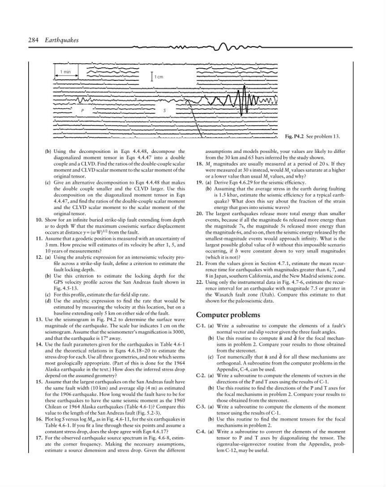
Fig. P4.2 See problem 13.
(b) Using the decomposition in Eqn 4.4.48, decompose the
diagonalized moment tensor in Eqn 4.4.47 into a double
couple and a CLVD. Find the ratios of the double-couple scalar
moment and CLVD scalar moment to the scalar moment of the
original tensor.
(c) Give an alternative decomposition to Eqn 4.4.48 that makes
the double couple smaller and the CLVD larger. Use this
decomposition on the diagonalized moment tensor in Eqn
4.4.47, and find the ratios of the double-couple scalar moment
and the CLVD scalar moment to the scalar moment of the
original tensor.
10. Show for an infinite buried strike-slip fault extending from depth
w to depth W that the maximum coseismic surface displacement
occurs at distance y = (wW) 1/2 from the fault.
11. Assume that a geodetic position is measured with an uncertainty of
3 mm. How precise will estimates of its velocity be after 1, 5, and
10 years of measurements?
12. (a) Using the analytic expression for an interseismic velocity profile across a strike-slip fault, define a criterion to estimate the
fault locking depth.
(b) Use this criterion to estimate the locking depth for the
GPS velocity profile across the San Andreas fault shown in
Fig. 4.5-13.
(c) For this profile, estimate the far-field slip rate.
(d) Use the analytic expression to find the rate that would be
estimated by measuring the velocity at this location, but on a
baseline extending only 5 km on either side of the fault.
13. Use the seismogram in Fig. P4.2 to determine the surface wave
magnitude of the earthquake. The scale bar indicates 1 cm on the
seismogram. Assume that the seismometer’s magnification is 3000,
and that the earthquake is 17° away.
14. Use the fault parameters given for the earthquakes in Table 4.6-1
and the theoretical relations in Eqns 4.6.18–20 to estimate the
stress drop for each. Use all three geometries, and note which seems
most geologically appropriate. (Part of this is done for the 1964
Alaska earthquake in the text.) How does the inferred stress drop
depend on the assumed geometry?
15. Assume that the largest earthquakes on the San Andreas fault have
the same fault width (10 km) and average slip (4 m) as estimated
for the 1906 earthquake. How long would the fault have to be for
these earthquakes to have the same seismic moment as the 1960
Chilean or 1964 Alaska earthquakes (Table 4.6-1)? Compare this
value to the length of the San Andreas fault (Fig. 5.2-3).
16. Plot log S versus log M 0 , as in Fig. 4.6-11, for the six earthquakes in
Table 4.6-1. If you fit a line through these six points and assume a
constant stress drop, does the slope agree with Eqn 4.6.17?
17. For the observed earthquake source spectrum in Fig. 4.6-8, estimate the corner frequency. Making the necessary assumptions,
estimate a source dimension and stress drop. Given the different
assumptions and models possible, your values are likely to differ
from the 30 km and 65 bars inferred by the study shown.
18. M s magnitudes are usually measured at a period of 20 s. If they
were measured at 30 s instead, would M s values saturate at a higher
or a lower value than usual M s values, and why?
19. (a) Derive Eqn 4.6.29 for the seismic efficiency.
(b) Assuming that the average stress in the earth during faulting
is 1.5 kbar, estimate the seismic efficiency for a typical earthquake? What does this say about the fraction of the strain
energy that goes into seismic waves?
20. The largest earthquakes release more total energy than smaller
events, because if all the magnitude 6s released more energy than
the magnitude 7s, the magnitude 5s released more energy than
the magnitude 6s, and so on, then the seismic energy released by the
smallest-magnitude events would approach infinity. What is the
largest possible global value of b without this impossible scenario
occurring, if b were constant down to very small magnitudes
(which it is not)?
21. From the values given in Section 4.7.1, estimate the mean recurrence time for earthquakes with magnitudes greater than 6, 7, and
8 in Japan, southern California, and the New Madrid seismic zone.
22. Using only the instrumental data in Fig. 4.7-6, estimate the recurrence interval for an earthquake with magnitude 7.5 or greater in
the Wasatch fault zone (Utah). Compare this estimate to that
shown for the paleoseismic data.
Computer problems
C-1. (a) Write a subroutine to compute the elements of a fault’s
normal vector and slip vector given the three fault angles.
(b) Use this routine to compute 4 and 2 for the focal mechanisms in problem 2. Compare your results to those obtained
from the stereonet.
(c) Test numerically that 4 and 2 for all these mechanisms are
orthogonal. A subroutine from the computer problems in the
Appendix, C-4, can be used.
C-2. (a) Write a subroutine to compute the elements of vectors in the
directions of the P and T axes using the results of C-1.
(b) Use this routine to find the directions of the P and T axes for
the focal mechanisms in problem 2. Compare your results to
those obtained from the stereonet.
C-3. (a) Write a subroutine to compute the elements of the moment
tensor using the results of C-1.
(b) Use this routine to find the moment tensors for the focal
mechanisms in problem 2.
C-4. (a) Write a subroutine to convert the elements of the moment
tensor to P and T axes by diagonalizing the tensor. The
eigenvalue–eigenvector routine from the Appendix, problem C-12, may be useful.
1 min
1 cm
S
P
Fig. P4.2 See problem 13.
(b) Using the decomposition in Eqn 4.4.48, decompose the
diagonalized moment tensor in Eqn 4.4.47 into a double
couple and a CLVD. Find the ratios of the double-couple scalar
moment and CLVD scalar moment to the scalar moment of the
original tensor.
(c) Give an alternative decomposition to Eqn 4.4.48 that makes
the double couple smaller and the CLVD larger. Use this
decomposition on the diagonalized moment tensor in Eqn
4.4.47, and find the ratios of the double-couple scalar moment
and the CLVD scalar moment to the scalar moment of the
original tensor.
10. Show for an infinite buried strike-slip fault extending from depth
w to depth W that the maximum coseismic surface displacement
occurs at distance y = (wW) 1/2 from the fault.
11. Assume that a geodetic position is measured with an uncertainty of
3 mm. How precise will estimates of its velocity be after 1, 5, and
10 years of measurements?
12. (a) Using the analytic expression for an interseismic velocity profile across a strike-slip fault, define a criterion to estimate the
fault locking depth.
(b) Use this criterion to estimate the locking depth for the
GPS velocity profile across the San Andreas fault shown in
Fig. 4.5-13.
(c) For this profile, estimate the far-field slip rate.
(d) Use the analytic expression to find the rate that would be
estimated by measuring the velocity at this location, but on a
baseline extending only 5 km on either side of the fault.
13. Use the seismogram in Fig. P4.2 to determine the surface wave
magnitude of the earthquake. The scale bar indicates 1 cm on the
seismogram. Assume that the seismometer’s magnification is 3000,
and that the earthquake is 17° away.
14. Use the fault parameters given for the earthquakes in Table 4.6-1
and the theoretical relations in Eqns 4.6.18–20 to estimate the
stress drop for each. Use all three geometries, and note which seems
most geologically appropriate. (Part of this is done for the 1964
Alaska earthquake in the text.) How does the inferred stress drop
depend on the assumed geometry?
15. Assume that the largest earthquakes on the San Andreas fault have
the same fault width (10 km) and average slip (4 m) as estimated
for the 1906 earthquake. How long would the fault have to be for
these earthquakes to have the same seismic moment as the 1960
Chilean or 1964 Alaska earthquakes (Table 4.6-1)? Compare this
value to the length of the San Andreas fault (Fig. 5.2-3).
16. Plot log S versus log M 0 , as in Fig. 4.6-11, for the six earthquakes in
Table 4.6-1. If you fit a line through these six points and assume a
constant stress drop, does the slope agree with Eqn 4.6.17?
17. For the observed earthquake source spectrum in Fig. 4.6-8, estimate the corner frequency. Making the necessary assumptions,
estimate a source dimension and stress drop. Given the different
assumptions and models possible, your values are likely to differ
from the 30 km and 65 bars inferred by the study shown.
18. M s magnitudes are usually measured at a period of 20 s. If they
were measured at 30 s instead, would M s values saturate at a higher
or a lower value than usual M s values, and why?
19. (a) Derive Eqn 4.6.29 for the seismic efficiency.
(b) Assuming that the average stress in the earth during faulting
is 1.5 kbar, estimate the seismic efficiency for a typical earthquake? What does this say about the fraction of the strain
energy that goes into seismic waves?
20. The largest earthquakes release more total energy than smaller
events, because if all the magnitude 6s released more energy than
the magnitude 7s, the magnitude 5s released more energy than
the magnitude 6s, and so on, then the seismic energy released by the
smallest-magnitude events would approach infinity. What is the
largest possible global value of b without this impossible scenario
occurring, if b were constant down to very small magnitudes
(which it is not)?
21. From the values given in Section 4.7.1, estimate the mean recurrence time for earthquakes with magnitudes greater than 6, 7, and
8 in Japan, southern California, and the New Madrid seismic zone.
22. Using only the instrumental data in Fig. 4.7-6, estimate the recurrence interval for an earthquake with magnitude 7.5 or greater in
the Wasatch fault zone (Utah). Compare this estimate to that
shown for the paleoseismic data.
Computer problems
C-1. (a) Write a subroutine to compute the elements of a fault’s
normal vector and slip vector given the three fault angles.
(b) Use this routine to compute 4 and 2 for the focal mechanisms in problem 2. Compare your results to those obtained
from the stereonet.
(c) Test numerically that 4 and 2 for all these mechanisms are
orthogonal. A subroutine from the computer problems in the
Appendix, C-4, can be used.
C-2. (a) Write a subroutine to compute the elements of vectors in the
directions of the P and T axes using the results of C-1.
(b) Use this routine to find the directions of the P and T axes for
the focal mechanisms in problem 2. Compare your results to
those obtained from the stereonet.
C-3. (a) Write a subroutine to compute the elements of the moment
tensor using the results of C-1.
(b) Use this routine to find the moment tensors for the focal
mechanisms in problem 2.
C-4. (a) Write a subroutine to convert the elements of the moment
tensor to P and T axes by diagonalizing the tensor. The
eigenvalue–eigenvector routine from the Appendix, problem C-12, may be useful.