

246 Earthquakes
Krafla
Lateral
intrusion
Flank
eruption
Conduit
Magma source
region
Shallow
magma
chamber
−2 km
−10 km
Approximate scale
66N
65N
64N
Bárdarbunga
Grímsvötn
Vatnajökull
19W
18W
17W
16W
15W
14W
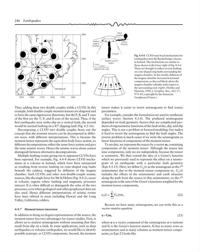
Fig. 4.4-8 CLVD-type focal mechanisms for
earthquakes near the Bardarbunga volcano
in Iceland. The mechanisms are similar to
those shown in the lower right of Fig. 4.4-6.
These are thought to reflect reverse faulting
on cone-shaped ring faults surrounding the
magma chamber. In this model, deflation of
the magma chamber increases horizontal
compression, so the roof block above the
magma chamber subsides with respect to
the surrounding rock (right). (Nettles and
Ekström, 1998. J. Geophys. Res., 103, 17,
973–83, copyright by the American
Geophysical Union.)
Thus, adding these two double couples yields a CLVD. In this
example, both double-couple moment tensors are diagonal and
so have the same eigenvector directions, but the P, B, and T axes
of the first are the T, P, and B axes of the second. Thus, if the
first earthquake were strike-slip on a vertical fault, the second
would be normal faulting on a 45°-dipping fault (Fig. 4.2-16).
Decomposing a CLVD into double couples bears out the
concept that the moment tensors can be decomposed in different ways, with different interpretations. This is because the
moment tensor represents the equivalent body force system, so
different decompositions reflect the same force system and give
the same seismic waves. Hence the seismic waves alone cannot
distinguish between alternative decompositions.
Multiple faulting events giving rise to apparent CLVDs have
been reported. For example, Fig. 4.4-8 shows CLVD mechanisms at a volcano in Iceland, which have been interpreted
as resulting from reverse faulting on cone-shaped ring faults
beneath the caldera, triggered by deflation of the magma
chamber. Such CLVDs and other non-double-couple seismic
sources, like the single force for Mt St Helens (Fig. 4.4-2), occur
in volcanic regions where faulting and magmatic processes
interact. It is often difficult to distinguish the roles of the two
processes, even when geological and other geophysical data are
also used. Hence different interpretations of seismic events
have been offered in areas including Hawaii and the Long
Valley, California, caldera.
4.4.7 Moment tensor inversion
In addition to being an elegant representation of the source, the
moment tensor has two advantages for source studies. First, it
allows us to analyze seismograms without assuming that they
result from slip on a fault. In some applications, such as deep
earthquakes or volcanic earthquakes, we would like to identify
possible isotropic or CLVD components. Second, the moment
tensor makes it easier to invert seismograms to find source
parameters.
For example, consider the formulation we used to synthesize
surface waves (Section 4.3.4). The predicted seismograms
depended on fault geometry factors that are complicated products of trigonometric functions of the fault strike, dip, and slip
angles. This is not a problem in forward modeling, but makes
it hard to invert the seismograms to find the fault angles. The
inverse problem is much easier if we write the seismograms as
linear functions of components of the moment tensor.
To see this, we represent the source by a vector m, containing
components of the moment tensor. Although the tensor has
nine components, only six are independent, because the tensor
is symmetric. We then extend the idea of a Green’s function
which we previously used to represent the effect on a seismogram of an earthquake with a particular fault geometry
(Eqn 4.3.15). Here, we define G ij (t) as the seismogram at the i
th
seismometer due to the moment tensor component m j . G ij (t)
includes the effects of the seismometer and earth structure
along the path from the source to this seismometer, so the i th
seismogram is the sum of the Green’s functions weighted by the
moment tensor components,
u i (t) =
G t m
ij
j
j
( ) .
=
∑
1
6
(22)
Because we have many seismograms, we can write this as a
vector–matrix equation
u = Gm,
(23)
where u is a vector composed of the seismograms at n stations
and G is the Green’s function matrix. G has as many rows as
seismometers and as many columns as moment tensor components, so Eqn 23 looks like
Krafla
Lateral
intrusion
Flank
eruption
Conduit
Magma source
region
Shallow
magma
chamber
−2 km
−10 km
Approximate scale
66N
65N
64N
Bárdarbunga
Grímsvötn
Vatnajökull
19W
18W
17W
16W
15W
14W
Fig. 4.4-8 CLVD-type focal mechanisms for
earthquakes near the Bardarbunga volcano
in Iceland. The mechanisms are similar to
those shown in the lower right of Fig. 4.4-6.
These are thought to reflect reverse faulting
on cone-shaped ring faults surrounding the
magma chamber. In this model, deflation of
the magma chamber increases horizontal
compression, so the roof block above the
magma chamber subsides with respect to
the surrounding rock (right). (Nettles and
Ekström, 1998. J. Geophys. Res., 103, 17,
973–83, copyright by the American
Geophysical Union.)
Thus, adding these two double couples yields a CLVD. In this
example, both double-couple moment tensors are diagonal and
so have the same eigenvector directions, but the P, B, and T axes
of the first are the T, P, and B axes of the second. Thus, if the
first earthquake were strike-slip on a vertical fault, the second
would be normal faulting on a 45°-dipping fault (Fig. 4.2-16).
Decomposing a CLVD into double couples bears out the
concept that the moment tensors can be decomposed in different ways, with different interpretations. This is because the
moment tensor represents the equivalent body force system, so
different decompositions reflect the same force system and give
the same seismic waves. Hence the seismic waves alone cannot
distinguish between alternative decompositions.
Multiple faulting events giving rise to apparent CLVDs have
been reported. For example, Fig. 4.4-8 shows CLVD mechanisms at a volcano in Iceland, which have been interpreted
as resulting from reverse faulting on cone-shaped ring faults
beneath the caldera, triggered by deflation of the magma
chamber. Such CLVDs and other non-double-couple seismic
sources, like the single force for Mt St Helens (Fig. 4.4-2), occur
in volcanic regions where faulting and magmatic processes
interact. It is often difficult to distinguish the roles of the two
processes, even when geological and other geophysical data are
also used. Hence different interpretations of seismic events
have been offered in areas including Hawaii and the Long
Valley, California, caldera.
4.4.7 Moment tensor inversion
In addition to being an elegant representation of the source, the
moment tensor has two advantages for source studies. First, it
allows us to analyze seismograms without assuming that they
result from slip on a fault. In some applications, such as deep
earthquakes or volcanic earthquakes, we would like to identify
possible isotropic or CLVD components. Second, the moment
tensor makes it easier to invert seismograms to find source
parameters.
For example, consider the formulation we used to synthesize
surface waves (Section 4.3.4). The predicted seismograms
depended on fault geometry factors that are complicated products of trigonometric functions of the fault strike, dip, and slip
angles. This is not a problem in forward modeling, but makes
it hard to invert the seismograms to find the fault angles. The
inverse problem is much easier if we write the seismograms as
linear functions of components of the moment tensor.
To see this, we represent the source by a vector m, containing
components of the moment tensor. Although the tensor has
nine components, only six are independent, because the tensor
is symmetric. We then extend the idea of a Green’s function
which we previously used to represent the effect on a seismogram of an earthquake with a particular fault geometry
(Eqn 4.3.15). Here, we define G ij (t) as the seismogram at the i
th
seismometer due to the moment tensor component m j . G ij (t)
includes the effects of the seismometer and earth structure
along the path from the source to this seismometer, so the i th
seismogram is the sum of the Green’s functions weighted by the
moment tensor components,
u i (t) =
G t m
ij
j
j
( ) .
=
∑
1
6
(22)
Because we have many seismograms, we can write this as a
vector–matrix equation
u = Gm,
(23)
where u is a vector composed of the seismograms at n stations
and G is the Green’s function matrix. G has as many rows as
seismometers and as many columns as moment tensor components, so Eqn 23 looks like