

Thus for two layers over a halfspace, the thickness of the
second layer is found by setting n = 2, so
h
h v
v
v
v
1
2
0
0
2
2
2 1 2
1
2
2
2 1 2
2 1
1
2 1
1
=
−
−
−
( /
/ )
( /
/ )
.
/
/
τ
(14)
A few examples illustrate some other complexities of refraction experiments. If the velocity increases with depth, the travel
time curve for the head wave at the top of each successive
layer has a shallower slope. By contrast, a low-velocity layer
(Fig. 3.2-8) does not cause a head wave, so the travel time curve
does not have a first arrival with the corresponding velocity,
and depths to interfaces calculated using Eqn 13 are incorrect.
Another possible problem occurs if a layer is thin or has a small
velocity contrast with the one below it. Although a head wave
results, it may never appear as a first arrival (Fig. 3.2-9), causing a blind zone that can be missed in the interpretation.
3.2.2 Dipping layer method
The refraction method can also be applied if the interfaces between layers are not horizontal. Conducting a reversed profile
yields the travel times for ray paths in both the down-dip
and the up-dip directions. This can be done using receivers on
either side of a source, sources on either side of a receiver,
or both. In this geometry, the depths to the interface below the
source and the receiver differ due to the dip angle, θ. Consider
3.2 Refraction seismology 123
Refraction data often show other arrivals in addition to P g ,
P n , and P m P. Figure 3.2-6 shows a record section that also contains head waves P i and P n 2 from boundaries within the crust
and the mantle and P i P, a reflection off a mid-crustal interface,
which is analogous to the P m P reflection off the Moho.
Such data require a model with multiple layers. Figure 3.2-7
shows a model in which a head wave arises at each interface
where the velocity increases with depth. The travel time curve
for a head wave at the top of the n th layer is a line with slope
1/v n , that can be extrapolated to its intercept on the t axis, τ n ,
and written
T x x v
H
n
n
n
( )
/
,
=
+τ
(11)
where, by analogy to the layer over the halfspace case (Eqn 9),
τ n
j
j
n
j
n
h v
v
=
−
=
−
∑ ( /
/ ) .
/
2
1
1
2
21 2
0
1
(12)
The thickness of successive layers can be found by starting with
the top layer, whose thickness h 0 is given by Eqn 9 or 10, and
continuing downward using the iterative formula
h
h v
v
v
v
n
n
j
j
n
j
n
n
n
−
=
−
−
=
−
−
−
∑
1
2
212
0
2
1
2
2 1 2
2
1
1
2 1
1
( /
/ )
( /
/ )
.
/
/
τ
(13)
Time
− X/6 (s)
+8
+7
+6
+5
+4
+3
+2
+1
0
−1
−2
−3
−4
−5
−6
80
Range (km)
P g
P n
P m P
90
100 110 120 130 140 150 160 170 180 190 200 210 220 230 240
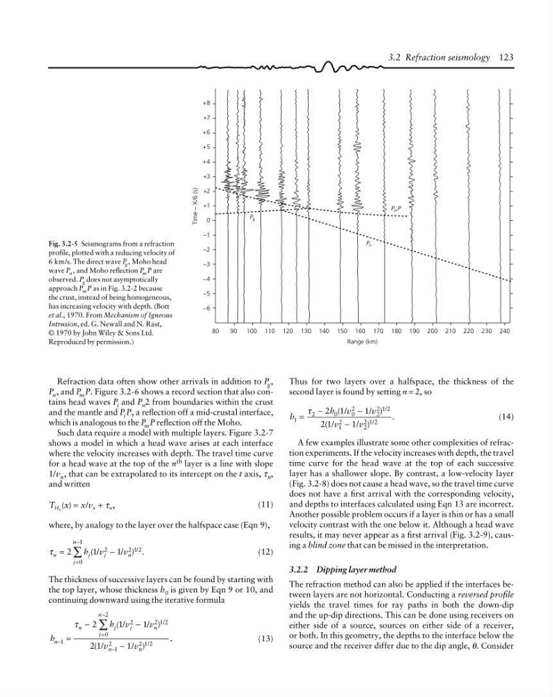
Fig. 3.2-5 Seismograms from a refraction
profile, plotted with a reducing velocity of
6 km/s. The direct wave P g , Moho head
wave P n , and Moho reflection P m P are
observed. P g does not asymptotically
approach P m P as in Fig. 3.2-2 because
the crust, instead of being homogeneous,
has increasing velocity with depth. (Bott
et al., 1970. From Mechanism of Igneous
Intrusion, ed. G. Newall and N. Rast,
© 1970 by John Wiley & Sons Ltd.
Reproduced by permission.)
second layer is found by setting n = 2, so
h
h v
v
v
v
1
2
0
0
2
2
2 1 2
1
2
2
2 1 2
2 1
1
2 1
1
=
−
−
−
( /
/ )
( /
/ )
.
/
/
τ
(14)
A few examples illustrate some other complexities of refraction experiments. If the velocity increases with depth, the travel
time curve for the head wave at the top of each successive
layer has a shallower slope. By contrast, a low-velocity layer
(Fig. 3.2-8) does not cause a head wave, so the travel time curve
does not have a first arrival with the corresponding velocity,
and depths to interfaces calculated using Eqn 13 are incorrect.
Another possible problem occurs if a layer is thin or has a small
velocity contrast with the one below it. Although a head wave
results, it may never appear as a first arrival (Fig. 3.2-9), causing a blind zone that can be missed in the interpretation.
3.2.2 Dipping layer method
The refraction method can also be applied if the interfaces between layers are not horizontal. Conducting a reversed profile
yields the travel times for ray paths in both the down-dip
and the up-dip directions. This can be done using receivers on
either side of a source, sources on either side of a receiver,
or both. In this geometry, the depths to the interface below the
source and the receiver differ due to the dip angle, θ. Consider
3.2 Refraction seismology 123
Refraction data often show other arrivals in addition to P g ,
P n , and P m P. Figure 3.2-6 shows a record section that also contains head waves P i and P n 2 from boundaries within the crust
and the mantle and P i P, a reflection off a mid-crustal interface,
which is analogous to the P m P reflection off the Moho.
Such data require a model with multiple layers. Figure 3.2-7
shows a model in which a head wave arises at each interface
where the velocity increases with depth. The travel time curve
for a head wave at the top of the n th layer is a line with slope
1/v n , that can be extrapolated to its intercept on the t axis, τ n ,
and written
T x x v
H
n
n
n
( )
/
,
=
+τ
(11)
where, by analogy to the layer over the halfspace case (Eqn 9),
τ n
j
j
n
j
n
h v
v
=
−
=
−
∑ ( /
/ ) .
/
2
1
1
2
21 2
0
1
(12)
The thickness of successive layers can be found by starting with
the top layer, whose thickness h 0 is given by Eqn 9 or 10, and
continuing downward using the iterative formula
h
h v
v
v
v
n
n
j
j
n
j
n
n
n
−
=
−
−
=
−
−
−
∑
1
2
212
0
2
1
2
2 1 2
2
1
1
2 1
1
( /
/ )
( /
/ )
.
/
/
τ
(13)
Time
− X/6 (s)
+8
+7
+6
+5
+4
+3
+2
+1
0
−1
−2
−3
−4
−5
−6
80
Range (km)
P g
P n
P m P
90
100 110 120 130 140 150 160 170 180 190 200 210 220 230 240
Fig. 3.2-5 Seismograms from a refraction
profile, plotted with a reducing velocity of
6 km/s. The direct wave P g , Moho head
wave P n , and Moho reflection P m P are
observed. P g does not asymptotically
approach P m P as in Fig. 3.2-2 because
the crust, instead of being homogeneous,
has increasing velocity with depth. (Bott
et al., 1970. From Mechanism of Igneous
Intrusion, ed. G. Newall and N. Rast,
© 1970 by John Wiley & Sons Ltd.
Reproduced by permission.)