

0
50
100
150
Time (hr)
Without splitting
Synthetic
Data
T = 53.8 min
0 S 2
Magnitude F(w)
400
300
200
100
0
−2
0
0 S 2 −1
+1
+2
0.0180 0.0185 0.0190
Observed
Synthetic
0
−2
Frequency (cycles/min)
+2
excite only the m = 0, ±1, and ±2 singlets because it radiates energy in a pattern with fourfold symmetry about the fault plane,
energy is transferred to the other singlets. Some coupling also
occurs between torsional and spheroidal modes, much as plane
P–SV and SH waves can be coupled at a dipping interface (Section 2.5.2). Hence torsional modes can contribute to the radial
displacement, which would not be possible for a SNREI earth.
As a result, some spectral peaks in Fig. 2.9-2 have several mode
labels, corresponding to modes with similar frequencies that
are coupled. These composite modes are called supermultiplets.
Although the theory of mode splitting and coupling is beyond our scope, it is worth noting that it is closely allied to conceptually similar problems in other branches of science. The
splitting due to earth’s rotation is similar to that for waves in
a rotating bowl of water, or to the Zeeman effect in atomic
physics, where spectral lines are split by a magnetic field. The
normal mode problems are addressed by exploring how perturbations to the equation of motion due to rotation, ellipticity,
lateral heterogeneity, etc. change the eigenfrequencies and
eigenfunctions from those for an unperturbed (SNREI) earth.
In summary, the peaks in a normal mode spectrum reflect
the combined effects of the earthquake, spherical and elastic
earth structure, attenuation, rotation, ellipticity, lateral heterogeneity, and anisotropy. As a result of extensive studies, these
effects are surprisingly well modeled, as shown by the good
(though not perfect) agreement between the synthetic and observed spectra in Fig. 2.9-2. Thus, as is so often the case, data
showing the deviations of the real earth from a simple model
are used to explore these deviations and better describe the real
earth.
Further reading
Further information about the topics of this chapter can be obtained from
many sources, a few of which are listed here. Basic wave concepts are discussed in books on wave propagation (e.g., Bland, 1988; French, 1971;
Main, 1978), classical mechanics (e.g., Feynman et al., 1963; Marion,
1970), and applied mathematics (e.g., Butkov, 1968; Morse and Feshbach,
1953; Menke and Abbott, 1990; Snieder, 2001). Introductions to topics
in continuum mechanics are given by Fung (1965, 1969) and Malvern
(1969). Fermat’s principle, Huygens’ principle, and diffraction are discussed in optics texts like Baker and Copson (1950) and Klein and Furtak
(1986).
Several introductory texts treat the seismological material in this chapter, including Ewing et al. (1957), Officer (1958), Richter (1958), Bullen
and Bolt (1985), Lay and Wallace (1995), Shearer (1999), and Udias
(1999). Advanced treatments beyond our discussions are given by Aki and
Richards (1980), Hudson (1980), Ben-Menahem and Singh (1981),
Lapwood and Usami (1981), Kennett (1983), Bath and Berkhout (1984),
and Dahlen and Tromp (1998).
A number of sources discuss specific topics that we address. Geller and
Stein (1978) discuss string examples like those used here, including of the
source term and of the modes of a non-uniform string. Young and Braile
(1976) review the solutions for reflection and transmission at a solid–solid
interface, and give the computer program used to calculate the energies in
Fig. 2.6-11 and 12. Madariaga (1972) derives the equivalence between
modes and traveling waves.
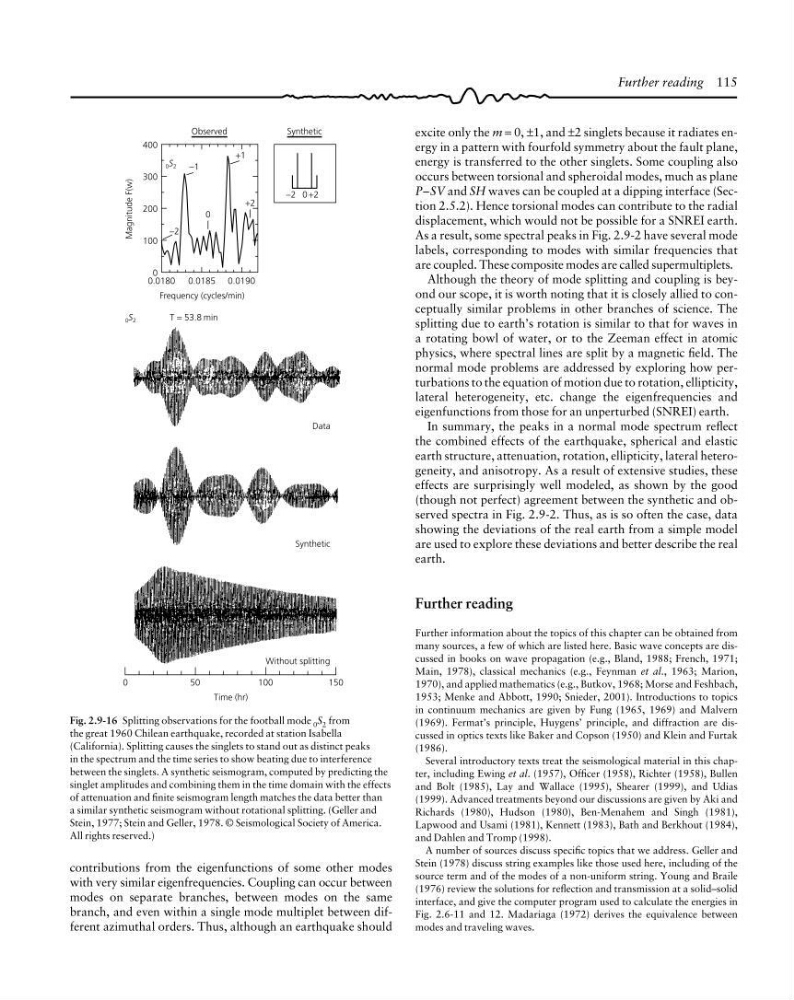
Fig. 2.9-16 Splitting observations for the football mode 0 S 2 from
the great 1960 Chilean earthquake, recorded at station Isabella
(California). Splitting causes the singlets to stand out as distinct peaks
in the spectrum and the time series to show beating due to interference
between the singlets. A synthetic seismogram, computed by predicting the
singlet amplitudes and combining them in the time domain with the effects
of attenuation and finite seismogram length matches the data better than
a similar synthetic seismogram without rotational splitting. (Geller and
Stein, 1977; Stein and Geller, 1978. © Seismological Society of America.
All rights reserved.)
contributions from the eigenfunctions of some other modes
with very similar eigenfrequencies. Coupling can occur between
modes on separate branches, between modes on the same
branch, and even within a single mode multiplet between different azimuthal orders. Thus, although an earthquake should
Further reading 115
50
100
150
Time (hr)
Without splitting
Synthetic
Data
T = 53.8 min
0 S 2
Magnitude F(w)
400
300
200
100
0
−2
0
0 S 2 −1
+1
+2
0.0180 0.0185 0.0190
Observed
Synthetic
0
−2
Frequency (cycles/min)
+2
excite only the m = 0, ±1, and ±2 singlets because it radiates energy in a pattern with fourfold symmetry about the fault plane,
energy is transferred to the other singlets. Some coupling also
occurs between torsional and spheroidal modes, much as plane
P–SV and SH waves can be coupled at a dipping interface (Section 2.5.2). Hence torsional modes can contribute to the radial
displacement, which would not be possible for a SNREI earth.
As a result, some spectral peaks in Fig. 2.9-2 have several mode
labels, corresponding to modes with similar frequencies that
are coupled. These composite modes are called supermultiplets.
Although the theory of mode splitting and coupling is beyond our scope, it is worth noting that it is closely allied to conceptually similar problems in other branches of science. The
splitting due to earth’s rotation is similar to that for waves in
a rotating bowl of water, or to the Zeeman effect in atomic
physics, where spectral lines are split by a magnetic field. The
normal mode problems are addressed by exploring how perturbations to the equation of motion due to rotation, ellipticity,
lateral heterogeneity, etc. change the eigenfrequencies and
eigenfunctions from those for an unperturbed (SNREI) earth.
In summary, the peaks in a normal mode spectrum reflect
the combined effects of the earthquake, spherical and elastic
earth structure, attenuation, rotation, ellipticity, lateral heterogeneity, and anisotropy. As a result of extensive studies, these
effects are surprisingly well modeled, as shown by the good
(though not perfect) agreement between the synthetic and observed spectra in Fig. 2.9-2. Thus, as is so often the case, data
showing the deviations of the real earth from a simple model
are used to explore these deviations and better describe the real
earth.
Further reading
Further information about the topics of this chapter can be obtained from
many sources, a few of which are listed here. Basic wave concepts are discussed in books on wave propagation (e.g., Bland, 1988; French, 1971;
Main, 1978), classical mechanics (e.g., Feynman et al., 1963; Marion,
1970), and applied mathematics (e.g., Butkov, 1968; Morse and Feshbach,
1953; Menke and Abbott, 1990; Snieder, 2001). Introductions to topics
in continuum mechanics are given by Fung (1965, 1969) and Malvern
(1969). Fermat’s principle, Huygens’ principle, and diffraction are discussed in optics texts like Baker and Copson (1950) and Klein and Furtak
(1986).
Several introductory texts treat the seismological material in this chapter, including Ewing et al. (1957), Officer (1958), Richter (1958), Bullen
and Bolt (1985), Lay and Wallace (1995), Shearer (1999), and Udias
(1999). Advanced treatments beyond our discussions are given by Aki and
Richards (1980), Hudson (1980), Ben-Menahem and Singh (1981),
Lapwood and Usami (1981), Kennett (1983), Bath and Berkhout (1984),
and Dahlen and Tromp (1998).
A number of sources discuss specific topics that we address. Geller and
Stein (1978) discuss string examples like those used here, including of the
source term and of the modes of a non-uniform string. Young and Braile
(1976) review the solutions for reflection and transmission at a solid–solid
interface, and give the computer program used to calculate the energies in
Fig. 2.6-11 and 12. Madariaga (1972) derives the equivalence between
modes and traveling waves.
Fig. 2.9-16 Splitting observations for the football mode 0 S 2 from
the great 1960 Chilean earthquake, recorded at station Isabella
(California). Splitting causes the singlets to stand out as distinct peaks
in the spectrum and the time series to show beating due to interference
between the singlets. A synthetic seismogram, computed by predicting the
singlet amplitudes and combining them in the time domain with the effects
of attenuation and finite seismogram length matches the data better than
a similar synthetic seismogram without rotational splitting. (Geller and
Stein, 1977; Stein and Geller, 1978. © Seismological Society of America.
All rights reserved.)
contributions from the eigenfunctions of some other modes
with very similar eigenfrequencies. Coupling can occur between
modes on separate branches, between modes on the same
branch, and even within a single mode multiplet between different azimuthal orders. Thus, although an earthquake should
Further reading 115