

82
P. Lazo et al.
45
40
35
30
25
20
15
10
5
1
11
10
9
8
7
6
5
4
3
2
MAPE 33.3049
MAD
1.4371
MSD
3.0160
Accuracy Measures
n
Br
Actual
Fits
Variable
Spatial Analysis Plot for Br
Linear Trend Model
Br = 6.658 - 0.0699×n
45
40
35
30
25
20
15
10
5
1
8
7
6
5
4
3
2
1
0
MAPE 72.5603
MAD
0.6909
MSD
1.5603
Accuracy Measures
n
I
Actual
Fits
Variable
Spatial Analysis Plot for I
Linear Trend Model
I = 1.569 + 0.0034×n
a.
b.
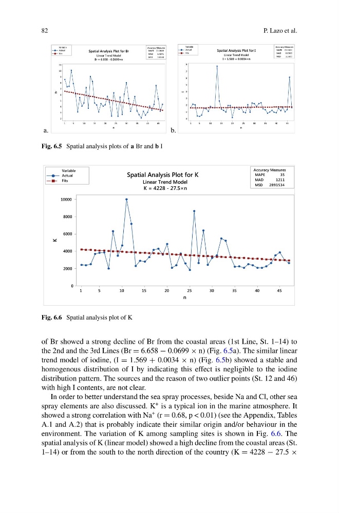
Fig. 6.5 Spatial analysis plots of a Br and b I
45
40
35
30
25
20
15
10
5
1
10000
8000
6000
4000
2000
0
MAPE
35
MAD
1211
MSD
2891534
Accuracy Measures
n
K
Actual
Fits
Variable
Spatial Analysis Plot for K
Linear Trend Model
K = 4228 - 27.5×n
Fig. 6.6 Spatial analysis plot of K
of Br showed a strong decline of Br from the coastal areas (1st Line, St. 1–14) to
the 2nd and the 3rd Lines (Br = 6.658 − 0.0699 × n) (Fig. 6.5a). The similar linear
trend model of iodine, (I = 1.569 + 0.0034 × n) (Fig. 6.5b) showed a stable and
homogenous distribution of I by indicating this effect is negligible to the iodine
distribution pattern. The sources and the reason of two outlier points (St. 12 and 46)
with high I contents, are not clear.
In order to better understand the sea spray processes, beside Na and Cl, other sea
spray elements are also discussed. K
+ is a typical ion in the marine atmosphere. It
showed a strong correlation with Na
+ (r = 0.68, p < 0.01) (see the Appendix, Tables
A.1 and A.2) that is probably indicate their similar origin and/or behaviour in the
environment. The variation of K among sampling sites is shown in Fig. 6.6. The
spatial analysis of K (linear model) showed a high decline from the coastal areas (St.
1–14) or from the south to the north direction of the country (K = 4228 − 27.5 ×
P. Lazo et al.
45
40
35
30
25
20
15
10
5
1
11
10
9
8
7
6
5
4
3
2
MAPE 33.3049
MAD
1.4371
MSD
3.0160
Accuracy Measures
n
Br
Actual
Fits
Variable
Spatial Analysis Plot for Br
Linear Trend Model
Br = 6.658 - 0.0699×n
45
40
35
30
25
20
15
10
5
1
8
7
6
5
4
3
2
1
0
MAPE 72.5603
MAD
0.6909
MSD
1.5603
Accuracy Measures
n
I
Actual
Fits
Variable
Spatial Analysis Plot for I
Linear Trend Model
I = 1.569 + 0.0034×n
a.
b.
Fig. 6.5 Spatial analysis plots of a Br and b I
45
40
35
30
25
20
15
10
5
1
10000
8000
6000
4000
2000
0
MAPE
35
MAD
1211
MSD
2891534
Accuracy Measures
n
K
Actual
Fits
Variable
Spatial Analysis Plot for K
Linear Trend Model
K = 4228 - 27.5×n
Fig. 6.6 Spatial analysis plot of K
of Br showed a strong decline of Br from the coastal areas (1st Line, St. 1–14) to
the 2nd and the 3rd Lines (Br = 6.658 − 0.0699 × n) (Fig. 6.5a). The similar linear
trend model of iodine, (I = 1.569 + 0.0034 × n) (Fig. 6.5b) showed a stable and
homogenous distribution of I by indicating this effect is negligible to the iodine
distribution pattern. The sources and the reason of two outlier points (St. 12 and 46)
with high I contents, are not clear.
In order to better understand the sea spray processes, beside Na and Cl, other sea
spray elements are also discussed. K
+ is a typical ion in the marine atmosphere. It
showed a strong correlation with Na
+ (r = 0.68, p < 0.01) (see the Appendix, Tables
A.1 and A.2) that is probably indicate their similar origin and/or behaviour in the
environment. The variation of K among sampling sites is shown in Fig. 6.6. The
spatial analysis of K (linear model) showed a high decline from the coastal areas (St.
1–14) or from the south to the north direction of the country (K = 4228 − 27.5 ×