

over a limited number of monitoring sites. This reduces the error in spatially variant
data rendering more accuracy to the geostatistical interpolation caused by uneven
spatial distribution of monitors. Also remotely sensed data of high resolution offers
tremendous spatial coverage suitable for regional air quality monitoring, pollution
event warning and environmental health studies.
5 Conclusion
In this paper, several spatial tools to quantify the effects of air quality on health have
been presented. The major challenge involved in the study of spatial exposure
assessment is the collection of the precise air quality information and the representative health data as they need to be scaled to a single spatial unit in order to apply
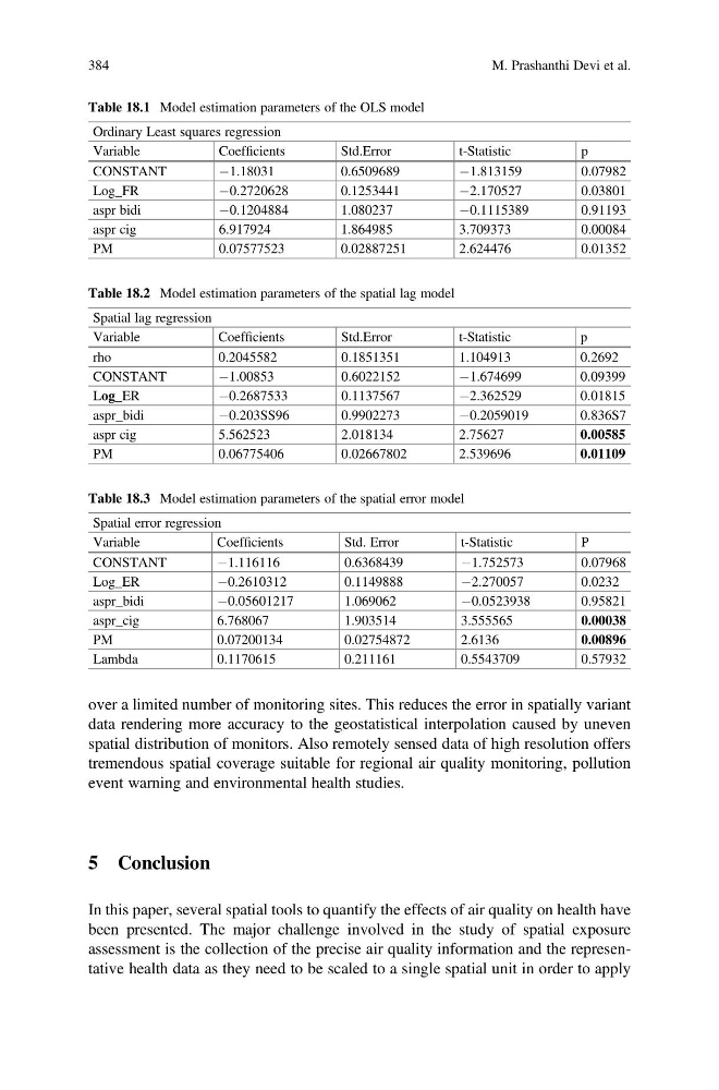
Table 18.1 Model estimation parameters of the OLS model
Ordinary Least squares regression
Variable
Coefficients
Std.Error
t-Statistic
p
CONSTANT
À1.18031
0.6509689
À1.813159
0.07982
Log_FR
À0.2720628
0.1253441
À2.170527
0.03801
aspr bidi
À0.1204884
1.080237
À0.1115389
0.91193
aspr cig
6.917924
1.864985
3.709373
0.00084
PM
0.07577523
0.02887251
2.624476
0.01352
Table 18.2 Model estimation parameters of the spatial lag model
Spatial lag regression
Variable
Coefficients
Std.Error
t-Statistic
p
rho
0.2045582
0.1851351
1.104913
0.2692
CONSTANT
À1.00853
0.6022152
À1.674699
0.09399
Log_ER
À0.2687533
0.1137567
À2.362529
0.01815
aspr_bidi
À0.203SS96
0.9902273
À0.2059019
0.836S7
aspr cig
5.562523
2.018134
2.75627
0.00585
PM
0.06775406
0.02667802
2.539696
0.01109
Table 18.3 Model estimation parameters of the spatial error model
Spatial error regression
Variable
Coefficients
Std. Error
t-Statistic
P
CONSTANT
À1.116116
0.6368439
À1.752573
0.07968
Log_ER
À0.2610312
0.1149888
À2.270057
0.0232
aspr_bidi
À0.05601217
1.069062
À0.0523938
0.95821
aspr_cig
6.768067
1.903514
3.555565
0.00038
PM
0.07200134
0.02754872
2.6136
0.00896
Lambda
0.1170615
0.211161
0.5543709
0.57932
384
M. Prashanthi Devi et al.
data rendering more accuracy to the geostatistical interpolation caused by uneven
spatial distribution of monitors. Also remotely sensed data of high resolution offers
tremendous spatial coverage suitable for regional air quality monitoring, pollution
event warning and environmental health studies.
5 Conclusion
In this paper, several spatial tools to quantify the effects of air quality on health have
been presented. The major challenge involved in the study of spatial exposure
assessment is the collection of the precise air quality information and the representative health data as they need to be scaled to a single spatial unit in order to apply
Table 18.1 Model estimation parameters of the OLS model
Ordinary Least squares regression
Variable
Coefficients
Std.Error
t-Statistic
p
CONSTANT
À1.18031
0.6509689
À1.813159
0.07982
Log_FR
À0.2720628
0.1253441
À2.170527
0.03801
aspr bidi
À0.1204884
1.080237
À0.1115389
0.91193
aspr cig
6.917924
1.864985
3.709373
0.00084
PM
0.07577523
0.02887251
2.624476
0.01352
Table 18.2 Model estimation parameters of the spatial lag model
Spatial lag regression
Variable
Coefficients
Std.Error
t-Statistic
p
rho
0.2045582
0.1851351
1.104913
0.2692
CONSTANT
À1.00853
0.6022152
À1.674699
0.09399
Log_ER
À0.2687533
0.1137567
À2.362529
0.01815
aspr_bidi
À0.203SS96
0.9902273
À0.2059019
0.836S7
aspr cig
5.562523
2.018134
2.75627
0.00585
PM
0.06775406
0.02667802
2.539696
0.01109
Table 18.3 Model estimation parameters of the spatial error model
Spatial error regression
Variable
Coefficients
Std. Error
t-Statistic
P
CONSTANT
À1.116116
0.6368439
À1.752573
0.07968
Log_ER
À0.2610312
0.1149888
À2.270057
0.0232
aspr_bidi
À0.05601217
1.069062
À0.0523938
0.95821
aspr_cig
6.768067
1.903514
3.555565
0.00038
PM
0.07200134
0.02754872
2.6136
0.00896
Lambda
0.1170615
0.211161
0.5543709
0.57932
384
M. Prashanthi Devi et al.