

with reflectance, satellite imagery can be utilized to plan and manage in situ
suspended solid sampling program. The raw satellite imagery can be automatically
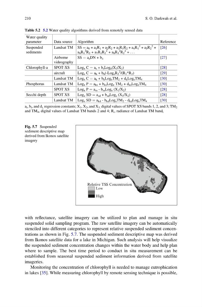
stenciled into different categories to represent relative suspended sediment concentrations as shown in Fig. 5.7. The suspended sediment descriptive map was derived
from Ikonos satellite data for a lake in Michigan. Such analysis will help visualize
the suspended sediment concentration changes within the water body and help plan
where to sample. The best time period to conduct in situ measurement can be
established from seasonal suspended sediment information derived from satellite
imageries.
Monitoring the concentration of chlorophyll is needed to manage eutrophication
in lakes [35]. While measuring chlorophyll by remote sensing technique is possible,
Table 5.2 5.2 Water quality algorithms derived from remotely sensed data
Water quality
parameter
Data source Algorithm
Reference
Suspended
sediments
Landsat TM SS ¼ a 0 + a 1 R 1 + a 2 R 2 + a 3 R 1 R 2 + a 4 R 1
2 + a 5 R 2
2 +
a 6 R 1
2
R 2 + a 7 R 1 R 2
2 + a 8 R 1
2
R 2
2 + . . .
[26]
Airborne
videography
SS ¼ a a DN + b a
[27]
Chlorophyll-a
SPOT-XS
Log e C ¼ a s + b s Log e (X 3 /X 2 )
[ 28]
aircraft
Log e C ¼ a h + b h (-Log e R 2
2
/(R 1 *R 3 )
[ 29]
Landsat TM Log e C ¼ a k + b k Log e TM 2 + d k Log e TM 4
[30]
Phosphorus
Landsat TM Log e P ¼ a ks + b ks Log e TM 2 + d ks Log e TM 4
[30]
SPOT XS
Log e P ¼ a ss - b ss Log e (X 1 /X 2 )
[ 28]
Secchi depth
SPOT XS
Log e SD ¼ a sd + b sd Log e (X 1 /X 2 )
[ 28]
Landsat TM Log e SD ¼ a kd - b kd Log e TM 2 - d kd Log e TM 4
[30]
a i , b i , and d i, regression constants; X 1 , X 2 , and X 3, digital values of SPOT XS bands 1, 2, and 3; TM 2
and TM 4 , digital values of Landsat TM bands 2 and 4; R i , radiance of Landsat TM band i
Low
High
Relative TSS Concentration
Fig. 5.7 Suspended
sediment descriptive map
derived from Ikonos satellite
imagery
210
S. O. Darkwah et al.
suspended solid sampling program. The raw satellite imagery can be automatically
stenciled into different categories to represent relative suspended sediment concentrations as shown in Fig. 5.7. The suspended sediment descriptive map was derived
from Ikonos satellite data for a lake in Michigan. Such analysis will help visualize
the suspended sediment concentration changes within the water body and help plan
where to sample. The best time period to conduct in situ measurement can be
established from seasonal suspended sediment information derived from satellite
imageries.
Monitoring the concentration of chlorophyll is needed to manage eutrophication
in lakes [35]. While measuring chlorophyll by remote sensing technique is possible,
Table 5.2 5.2 Water quality algorithms derived from remotely sensed data
Water quality
parameter
Data source Algorithm
Reference
Suspended
sediments
Landsat TM SS ¼ a 0 + a 1 R 1 + a 2 R 2 + a 3 R 1 R 2 + a 4 R 1
2 + a 5 R 2
2 +
a 6 R 1
2
R 2 + a 7 R 1 R 2
2 + a 8 R 1
2
R 2
2 + . . .
[26]
Airborne
videography
SS ¼ a a DN + b a
[27]
Chlorophyll-a
SPOT-XS
Log e C ¼ a s + b s Log e (X 3 /X 2 )
[ 28]
aircraft
Log e C ¼ a h + b h (-Log e R 2
2
/(R 1 *R 3 )
[ 29]
Landsat TM Log e C ¼ a k + b k Log e TM 2 + d k Log e TM 4
[30]
Phosphorus
Landsat TM Log e P ¼ a ks + b ks Log e TM 2 + d ks Log e TM 4
[30]
SPOT XS
Log e P ¼ a ss - b ss Log e (X 1 /X 2 )
[ 28]
Secchi depth
SPOT XS
Log e SD ¼ a sd + b sd Log e (X 1 /X 2 )
[ 28]
Landsat TM Log e SD ¼ a kd - b kd Log e TM 2 - d kd Log e TM 4
[30]
a i , b i , and d i, regression constants; X 1 , X 2 , and X 3, digital values of SPOT XS bands 1, 2, and 3; TM 2
and TM 4 , digital values of Landsat TM bands 2 and 4; R i , radiance of Landsat TM band i
Low
High
Relative TSS Concentration
Fig. 5.7 Suspended
sediment descriptive map
derived from Ikonos satellite
imagery
210
S. O. Darkwah et al.