

[20]. Darkwah and Scoville [21] used a times series of Landsat TM and MSS to
document the dynamic changes in the Kalamazoo River basin in Michigan. The GIS
and remote sensing approach to floodplain mapping presents a quick and operational
method for flood mapping. The technique involves using multi-temporal imageries
and a basic mathematical logic to identify the extent and amount of flood. The
mathematical operations usually performed include addition, subtraction, multiplication, and division. The multi-temporal change detection approach usually requires
a low flow image dataset (base image data) and an image during the flood period
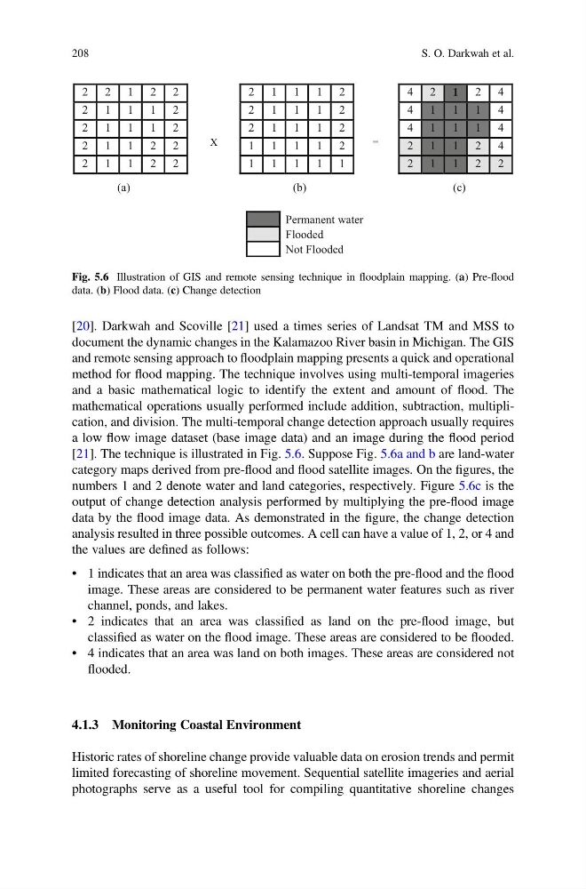
[21]. The technique is illustrated in Fig. 5.6. Suppose Fig. 5.6a and b are land-water
category maps derived from pre-flood and flood satellite images. On the figures, the
numbers 1 and 2 denote water and land categories, respectively. Figure 5.6c is the
output of change detection analysis performed by multiplying the pre-flood image
data by the flood image data. As demonstrated in the figure, the change detection
analysis resulted in three possible outcomes. A cell can have a value of 1, 2, or 4 and
the values are defined as follows:
• 1 indicates that an area was classified as water on both the pre-flood and the flood
image. These areas are considered to be permanent water features such as river
channel, ponds, and lakes.
• 2 indicates that an area was classified as land on the pre-flood image, but
classified as water on the flood image. These areas are considered to be flooded.
• 4 indicates that an area was land on both images. These areas are considered not
flooded.
4.1.3 Monitoring Coastal Environment
Historic rates of shoreline change provide valuable data on erosion trends and permit
limited forecasting of shoreline movement. Sequential satellite imageries and aerial
photographs serve as a useful tool for compiling quantitative shoreline changes
X
=
Permanent water
(a)
(b)
(c)
Flooded
Not Flooded
2 2 1 2 2
2 1 1 1 2
2 1 1 1 2
2 1 1 2 2
2 1 1 2 2
2 1 1 1 2
2 1 1 1 2
2 1 1 1 2
1 1 1 1 2
1 1 1 1 1
4 2 1 2 4
4 1 1 1 4
4 1 1 1 4
2 1 1 2 4
2 1 1 2 2
Fig. 5.6 Illustration of GIS and remote sensing technique in floodplain mapping. (a) Pre-flood
data. (b) Flood data. (c) Change detection
208
S. O. Darkwah et al.
document the dynamic changes in the Kalamazoo River basin in Michigan. The GIS
and remote sensing approach to floodplain mapping presents a quick and operational
method for flood mapping. The technique involves using multi-temporal imageries
and a basic mathematical logic to identify the extent and amount of flood. The
mathematical operations usually performed include addition, subtraction, multiplication, and division. The multi-temporal change detection approach usually requires
a low flow image dataset (base image data) and an image during the flood period
[21]. The technique is illustrated in Fig. 5.6. Suppose Fig. 5.6a and b are land-water
category maps derived from pre-flood and flood satellite images. On the figures, the
numbers 1 and 2 denote water and land categories, respectively. Figure 5.6c is the
output of change detection analysis performed by multiplying the pre-flood image
data by the flood image data. As demonstrated in the figure, the change detection
analysis resulted in three possible outcomes. A cell can have a value of 1, 2, or 4 and
the values are defined as follows:
• 1 indicates that an area was classified as water on both the pre-flood and the flood
image. These areas are considered to be permanent water features such as river
channel, ponds, and lakes.
• 2 indicates that an area was classified as land on the pre-flood image, but
classified as water on the flood image. These areas are considered to be flooded.
• 4 indicates that an area was land on both images. These areas are considered not
flooded.
4.1.3 Monitoring Coastal Environment
Historic rates of shoreline change provide valuable data on erosion trends and permit
limited forecasting of shoreline movement. Sequential satellite imageries and aerial
photographs serve as a useful tool for compiling quantitative shoreline changes
X
=
Permanent water
(a)
(b)
(c)
Flooded
Not Flooded
2 2 1 2 2
2 1 1 1 2
2 1 1 1 2
2 1 1 2 2
2 1 1 2 2
2 1 1 1 2
2 1 1 1 2
2 1 1 1 2
1 1 1 1 2
1 1 1 1 1
4 2 1 2 4
4 1 1 1 4
4 1 1 1 4
2 1 1 2 4
2 1 1 2 2
Fig. 5.6 Illustration of GIS and remote sensing technique in floodplain mapping. (a) Pre-flood
data. (b) Flood data. (c) Change detection
208
S. O. Darkwah et al.