

division is used here because instream models are not used routinely in pollution
incident assessments unless they have been calibrated specifically for that purpose.
The dimensions simulated by a particular model will provide information on both the
complexity of a model and also on its suitability to specific applications. A zerodimensional (0D) model does not represent the processes of dispersion of contaminants in any direction, but simply represents the volumes and concentrations
assuming that the water body is completely and instantaneously mixed. A onedimensional (1D) model represents the water flow and the advection and dispersion
of solutes in just one direction (i.e., downstream in a river model) and so the stream is
assumed to be completely (and instantaneously) mixed across its width and depth.
Following from this, a two dimensional (2D) model will either simulate dispersion
across the width or the depth of the stream, but not both. A width-averaged model is
often used in simulating thermal stratification of deepwater bodies or when there
may be layers of salt and freshwater at different depths in estuaries. Depth-averaged
models are useful when the river is broad and shallow such that stratification is
limited, but dispersion across the width of the river is slow. Three-dimensional
(3D) models account for the water flows and solute transport in all directions.
These models are highly sophisticated, and 3D water quality models are usually
reserved for large (i.e., deep and wide) estuaries where the mixing patterns are
complex (Fig. 3.9).
x – axis
x(t) =
x max =
t – axis
t max =
log(e)
2M 2 p · e
4M 2 p · D
–2D · t In(4M 2 pD · t)
1
t 0 =
4M 2 p · D · e
1
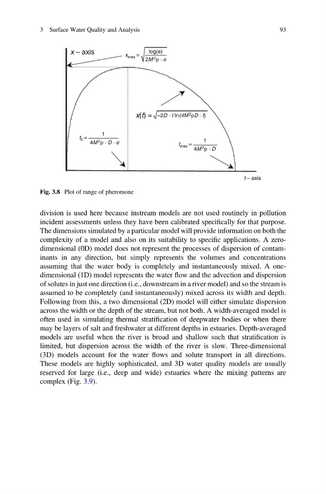
Fig. 3.8 Plot of range of pheromone
3 Surface Water Quality and Analysis
93
incident assessments unless they have been calibrated specifically for that purpose.
The dimensions simulated by a particular model will provide information on both the
complexity of a model and also on its suitability to specific applications. A zerodimensional (0D) model does not represent the processes of dispersion of contaminants in any direction, but simply represents the volumes and concentrations
assuming that the water body is completely and instantaneously mixed. A onedimensional (1D) model represents the water flow and the advection and dispersion
of solutes in just one direction (i.e., downstream in a river model) and so the stream is
assumed to be completely (and instantaneously) mixed across its width and depth.
Following from this, a two dimensional (2D) model will either simulate dispersion
across the width or the depth of the stream, but not both. A width-averaged model is
often used in simulating thermal stratification of deepwater bodies or when there
may be layers of salt and freshwater at different depths in estuaries. Depth-averaged
models are useful when the river is broad and shallow such that stratification is
limited, but dispersion across the width of the river is slow. Three-dimensional
(3D) models account for the water flows and solute transport in all directions.
These models are highly sophisticated, and 3D water quality models are usually
reserved for large (i.e., deep and wide) estuaries where the mixing patterns are
complex (Fig. 3.9).
x – axis
x(t) =
x max =
t – axis
t max =
log(e)
2M 2 p · e
4M 2 p · D
–2D · t In(4M 2 pD · t)
1
t 0 =
4M 2 p · D · e
1
Fig. 3.8 Plot of range of pheromone
3 Surface Water Quality and Analysis
93