

3.6 Seafloor Compartment Functions
53
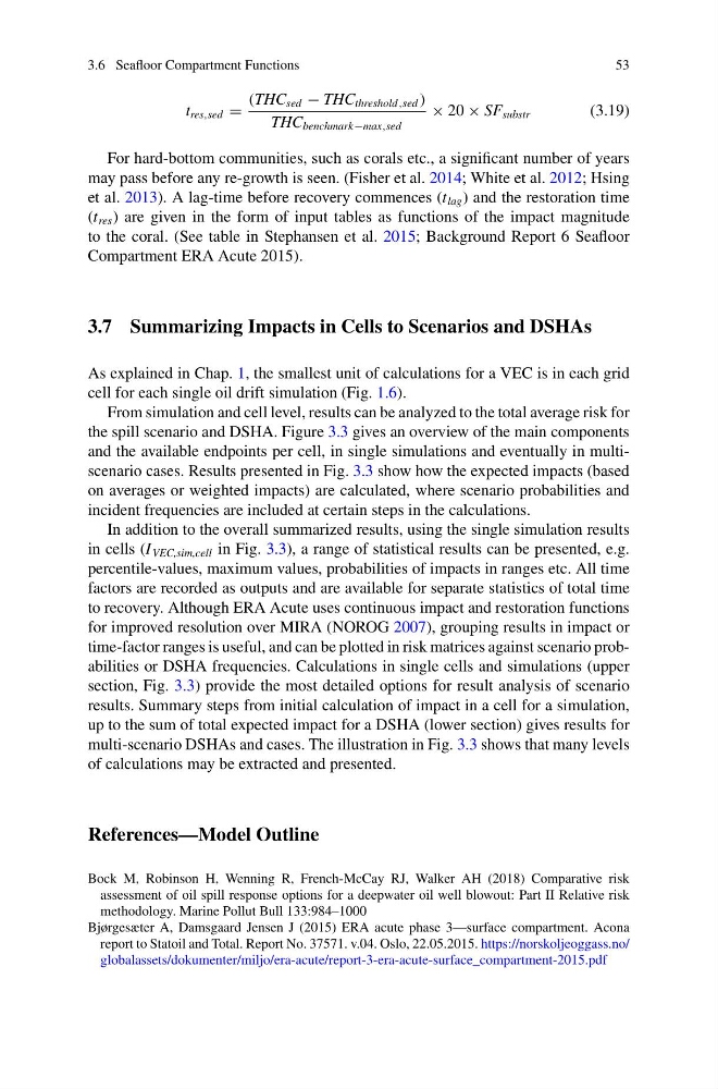
t res,sed =
(THC sed − THC threshold ,sed )
THC benchmark−max,sed
× 20 × SF substr
(3.19)
For hard-bottom communities, such as corals etc., a significant number of years
may pass before any re-growth is seen. (Fisher et al. 2014; White et al. 2012; Hsing
et al. 2013). A lag-time before recovery commences (t lag ) and the restoration time
(t res ) are given in the form of input tables as functions of the impact magnitude
to the coral. (See table in Stephansen et al. 2015; Background Report 6 Seafloor
Compartment ERA Acute 2015).
3.7 Summarizing Impacts in Cells to Scenarios and DSHAs
As explained in Chap. 1, the smallest unit of calculations for a VEC is in each grid
cell for each single oil drift simulation (Fig. 1.6).
From simulation and cell level, results can be analyzed to the total average risk for
the spill scenario and DSHA. Figure 3.3 gives an overview of the main components
and the available endpoints per cell, in single simulations and eventually in multiscenario cases. Results presented in Fig. 3.3 show how the expected impacts (based
on averages or weighted impacts) are calculated, where scenario probabilities and
incident frequencies are included at certain steps in the calculations.
In addition to the overall summarized results, using the single simulation results
in cells (I VEC,sim,cell in Fig. 3.3), a range of statistical results can be presented, e.g.
percentile-values, maximum values, probabilities of impacts in ranges etc. All time
factors are recorded as outputs and are available for separate statistics of total time
to recovery. Although ERA Acute uses continuous impact and restoration functions
for improved resolution over MIRA (NOROG 2007), grouping results in impact or
time-factor ranges is useful, and can be plotted in risk matrices against scenario probabilities or DSHA frequencies. Calculations in single cells and simulations (upper
section, Fig. 3.3) provide the most detailed options for result analysis of scenario
results. Summary steps from initial calculation of impact in a cell for a simulation,
up to the sum of total expected impact for a DSHA (lower section) gives results for
multi-scenario DSHAs and cases. The illustration in Fig. 3.3 shows that many levels
of calculations may be extracted and presented.
References—Model Outline
Bock M, Robinson H, Wenning R, French-McCay RJ, Walker AH (2018) Comparative risk
assessment of oil spill response options for a deepwater oil well blowout: Part II Relative risk
methodology. Marine Pollut Bull 133:984–1000
Bjørgesæter A, Damsgaard Jensen J (2015) ERA acute phase 3—surface compartment. Acona
report to Statoil and Total. Report No. 37571. v.04. Oslo, 22.05.2015. https://norskoljeoggass.no/
globalassets/dokumenter/miljo/era-acute/report-3-era-acute-surface_compartment-2015.pdf
53
t res,sed =
(THC sed − THC threshold ,sed )
THC benchmark−max,sed
× 20 × SF substr
(3.19)
For hard-bottom communities, such as corals etc., a significant number of years
may pass before any re-growth is seen. (Fisher et al. 2014; White et al. 2012; Hsing
et al. 2013). A lag-time before recovery commences (t lag ) and the restoration time
(t res ) are given in the form of input tables as functions of the impact magnitude
to the coral. (See table in Stephansen et al. 2015; Background Report 6 Seafloor
Compartment ERA Acute 2015).
3.7 Summarizing Impacts in Cells to Scenarios and DSHAs
As explained in Chap. 1, the smallest unit of calculations for a VEC is in each grid
cell for each single oil drift simulation (Fig. 1.6).
From simulation and cell level, results can be analyzed to the total average risk for
the spill scenario and DSHA. Figure 3.3 gives an overview of the main components
and the available endpoints per cell, in single simulations and eventually in multiscenario cases. Results presented in Fig. 3.3 show how the expected impacts (based
on averages or weighted impacts) are calculated, where scenario probabilities and
incident frequencies are included at certain steps in the calculations.
In addition to the overall summarized results, using the single simulation results
in cells (I VEC,sim,cell in Fig. 3.3), a range of statistical results can be presented, e.g.
percentile-values, maximum values, probabilities of impacts in ranges etc. All time
factors are recorded as outputs and are available for separate statistics of total time
to recovery. Although ERA Acute uses continuous impact and restoration functions
for improved resolution over MIRA (NOROG 2007), grouping results in impact or
time-factor ranges is useful, and can be plotted in risk matrices against scenario probabilities or DSHA frequencies. Calculations in single cells and simulations (upper
section, Fig. 3.3) provide the most detailed options for result analysis of scenario
results. Summary steps from initial calculation of impact in a cell for a simulation,
up to the sum of total expected impact for a DSHA (lower section) gives results for
multi-scenario DSHAs and cases. The illustration in Fig. 3.3 shows that many levels
of calculations may be extracted and presented.
References—Model Outline
Bock M, Robinson H, Wenning R, French-McCay RJ, Walker AH (2018) Comparative risk
assessment of oil spill response options for a deepwater oil well blowout: Part II Relative risk
methodology. Marine Pollut Bull 133:984–1000
Bjørgesæter A, Damsgaard Jensen J (2015) ERA acute phase 3—surface compartment. Acona
report to Statoil and Total. Report No. 37571. v.04. Oslo, 22.05.2015. https://norskoljeoggass.no/
globalassets/dokumenter/miljo/era-acute/report-3-era-acute-surface_compartment-2015.pdf