

52
3 An ERA Acute Model Overview
sponges THC WC is currently used directly to determine plet WC,SF using an SSDcurve derived by Nilsen et al. 2006, pending improved stochastic modelling of timeaveraged mortality directly in the lower water column using the preferred method
for water column resources (see 3.6.1).
Species that ingest sediment particles are exposed both externally (plet IW or
plet WC,SF ) and with added lethality from plet Ing . Seven feeding modes are identified based on biological criteria, which are assigned to four essential exposure mode
combinations: Exposure through water column (WC) (epifauna) or IW (infauna) and
any of these with ingestion (Ing) for deposit feeders.
VEC data are prepared either as single-species data or substrate-based data
community data with a feeding mode. If accurate data for distributions of feeding
modes within a community can be found, it is possible to assign community VECs
with a combination of fractions of feeding modes in a community contributing to
the calculation (See Stephansen et al. 2015). For species that are partially infaunal,
partially epifaunal, such as e.g. seapens, these may be ascribed an additive effect of
both WC and IW exposure by using both modes to define exposure. The calculator
will then summarize the two p let -values to an additive effect.
3.6.2 Time Factors and Recovery Modelling
In the seafloor compartment, the time factors are included in the impact calculation
for each cell and simulation before the results are summarized and statistics are
presented. Impact time, t imp is default set to 1 year to cover an annual cycle. For soft
substrates, the lag-time, t lag,sed is set to 0 in the current soft substrate implementation,
assuming that restoration begins next reproductive cycle.
Restoration time, t res in soft substrates are calculated by a linear relationship
(Olsgård and Gray 1995) implemented as Eq. 3.19, between the amount of oil in
the sediment (THC sed ) above a threshold value (THC threshold,sed ) (currently 50 ppm,
Renaud et al. 2008) and the expected maximum concentration of THC resulting
from sedimentation of oil from an accidental release (THC benchmark-max,sed ). (currently
1000 ppm (Olsgård and Gray 1995). The average value of 20 years found in literature search (Renaud et al. 2008) is based on data from the North Sea (for which
sandy sediments are the “standard” substrate). For VECs (substrate communities)
with different recovery times than the average value of 20 years, a restoration timemodifying sensitivity factor (SF) is used to calculate t res (Eq. 3.19). The value of SF
is currently proposed to be calculated as the ratio of the TOC-content of the substrate
relative to the TOC-content of the sand substrate for which 20 years was found to be
the restoration time (“standard-substrate”) (Eq. 3.18, in Stephansen and Bjørgesæter
2018). RDF is calculated from the general Eq. 3.9 shared with Shoreline.
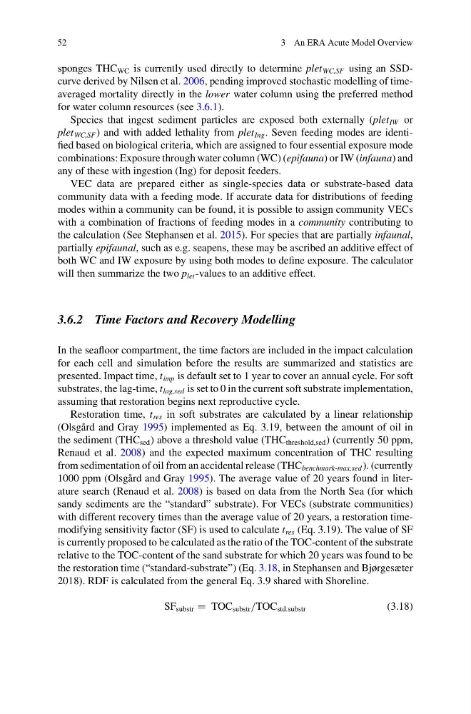
SF substr = TOC substr /TOC std.substr
(3.18)
3 An ERA Acute Model Overview
sponges THC WC is currently used directly to determine plet WC,SF using an SSDcurve derived by Nilsen et al. 2006, pending improved stochastic modelling of timeaveraged mortality directly in the lower water column using the preferred method
for water column resources (see 3.6.1).
Species that ingest sediment particles are exposed both externally (plet IW or
plet WC,SF ) and with added lethality from plet Ing . Seven feeding modes are identified based on biological criteria, which are assigned to four essential exposure mode
combinations: Exposure through water column (WC) (epifauna) or IW (infauna) and
any of these with ingestion (Ing) for deposit feeders.
VEC data are prepared either as single-species data or substrate-based data
community data with a feeding mode. If accurate data for distributions of feeding
modes within a community can be found, it is possible to assign community VECs
with a combination of fractions of feeding modes in a community contributing to
the calculation (See Stephansen et al. 2015). For species that are partially infaunal,
partially epifaunal, such as e.g. seapens, these may be ascribed an additive effect of
both WC and IW exposure by using both modes to define exposure. The calculator
will then summarize the two p let -values to an additive effect.
3.6.2 Time Factors and Recovery Modelling
In the seafloor compartment, the time factors are included in the impact calculation
for each cell and simulation before the results are summarized and statistics are
presented. Impact time, t imp is default set to 1 year to cover an annual cycle. For soft
substrates, the lag-time, t lag,sed is set to 0 in the current soft substrate implementation,
assuming that restoration begins next reproductive cycle.
Restoration time, t res in soft substrates are calculated by a linear relationship
(Olsgård and Gray 1995) implemented as Eq. 3.19, between the amount of oil in
the sediment (THC sed ) above a threshold value (THC threshold,sed ) (currently 50 ppm,
Renaud et al. 2008) and the expected maximum concentration of THC resulting
from sedimentation of oil from an accidental release (THC benchmark-max,sed ). (currently
1000 ppm (Olsgård and Gray 1995). The average value of 20 years found in literature search (Renaud et al. 2008) is based on data from the North Sea (for which
sandy sediments are the “standard” substrate). For VECs (substrate communities)
with different recovery times than the average value of 20 years, a restoration timemodifying sensitivity factor (SF) is used to calculate t res (Eq. 3.19). The value of SF
is currently proposed to be calculated as the ratio of the TOC-content of the substrate
relative to the TOC-content of the sand substrate for which 20 years was found to be
the restoration time (“standard-substrate”) (Eq. 3.18, in Stephansen and Bjørgesæter
2018). RDF is calculated from the general Eq. 3.9 shared with Shoreline.
SF substr = TOC substr /TOC std.substr
(3.18)