

2.3 Electronic Structures
31
with c ir being the MO coefficient and n the total number of the AO’s {χ r (r)}. Hence
ρ(r) in Eq. (2.12) is further decomposed into
ρ(r) =
occ
i
n i
n
r,s
c
∗
ir c is χ
∗
r (r)χ s (r)
(2.14)
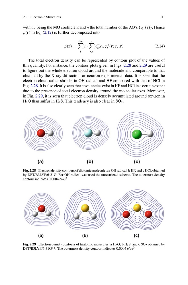
The total electron density can be represented by contour plot of the values of
this quantity. For instance, the contour plots given in Figs. 2.28 and 2.29 are useful
to figure out the whole electron cloud around the molecule and comparable to that
obtained by the X-ray diffraction or neutron experimental data. It is seen that the
electron cloud rather shrinks in OH radical and HF compared with that of HCl in
Fig. 2.28. It is also clearly seen that covalencies exist in HF and HCl in a certain extent
due to the presence of total electron density around the molecular axes. Moreover,
in Fig. 2.29, it is seen that electron cloud is densely accumulated around oxygen in
H 2 O than sulfur in H 2 S. This tendency is also clear in SO 2 .
Fig. 2.28 Electron density contours of diatomic molecules: a OH radical, b HF, and c HCl, obtained
by DFT/B3LYP/6-31G. For OH radical was used the unrestricted scheme. The outermost density
contour indicates 0.0004 e/au 3
Fig. 2.29 Electron density contours of triatomic molecules: a H 2 O, b H 2 S, and c SO 2 obtained by
DFT/B3LYP/6-31G**. The outermost density contour indicates 0.0004 e/au 3
31
with c ir being the MO coefficient and n the total number of the AO’s {χ r (r)}. Hence
ρ(r) in Eq. (2.12) is further decomposed into
ρ(r) =
occ
i
n i
n
r,s
c
∗
ir c is χ
∗
r (r)χ s (r)
(2.14)
The total electron density can be represented by contour plot of the values of
this quantity. For instance, the contour plots given in Figs. 2.28 and 2.29 are useful
to figure out the whole electron cloud around the molecule and comparable to that
obtained by the X-ray diffraction or neutron experimental data. It is seen that the
electron cloud rather shrinks in OH radical and HF compared with that of HCl in
Fig. 2.28. It is also clearly seen that covalencies exist in HF and HCl in a certain extent
due to the presence of total electron density around the molecular axes. Moreover,
in Fig. 2.29, it is seen that electron cloud is densely accumulated around oxygen in
H 2 O than sulfur in H 2 S. This tendency is also clear in SO 2 .
Fig. 2.28 Electron density contours of diatomic molecules: a OH radical, b HF, and c HCl, obtained
by DFT/B3LYP/6-31G. For OH radical was used the unrestricted scheme. The outermost density
contour indicates 0.0004 e/au 3
Fig. 2.29 Electron density contours of triatomic molecules: a H 2 O, b H 2 S, and c SO 2 obtained by
DFT/B3LYP/6-31G**. The outermost density contour indicates 0.0004 e/au 3