

140
3 Fundamentals of the Analysis Tools
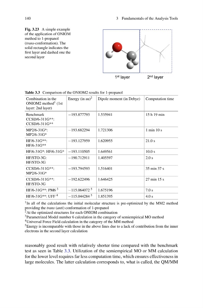
Fig. 3.23 A simple example
of the application of ONIOM
method to 1-propanol
(trans-conformation). The
solid rectangle indicates the
first layer and dashed one the
second layer
1 st layer
2 nd layer
Table 3.3 Comparison of the ONIOM2 results for 1-propanol
Combination in the
ONIOM2 method 1 (1st
layer: 2nd layer)
Energy (in au) 2 Dipole moment (in Debye) Computation time
Benchmark
CCSD/6-311G**:
CCSD/6-311G**
−193.877793
1.535941
15 h 19 min
MP2/6-31G*:
MP2/6-31G*
−193.682294
1.721306
1 min 10 s
HF/6-31G**:
HF/6-31G**
−193.127959
1.620955
21.0 s
HF/6-31G*: HF/6-31G* −193.110505
1.649561
10.0 s
HF/STO-3G:
HF/STO-3G
−190.712911
1.405597
2.0 s
CCSD/6-311G**:
MP2/6-31G*
−193.794593
1.516401
35 min 37 s
CCSD/6-311G**:
HF/STO-3G
−192.622496
1.646425
27 min 15 s
HF/6-31G**: PM6 3
−115.064072 5 1.675196
7.0 s
HF/6-31G**: UFF 4
−115.044284 5 1.851395
4.0 s
1 In all of the calculations the initial molecular structure is pre-optimized by the MM2 method
providing the trans (anti) conformation of 1-propanol
2 At the optimized structures for each ONIOM combination
3 Parametrized Model number 6 calculation in the category of semiempirical MO method
4 Universal Force Field calculation in the category of the MM method
5 Energy is incomparable with those in the above lines due to a lack of contribution from the inner
electrons in the second layer calculation
reasonably good result with relatively shorter time compared with the benchmark
test as seen in Table 3.3. Utilization of the semiempirical MO or MM calculation
for the lower level requires far less computation time, which ensures effectiveness in
large molecules. The latter calculation corresponds to, what is called, the QM/MM
3 Fundamentals of the Analysis Tools
Fig. 3.23 A simple example
of the application of ONIOM
method to 1-propanol
(trans-conformation). The
solid rectangle indicates the
first layer and dashed one the
second layer
1 st layer
2 nd layer
Table 3.3 Comparison of the ONIOM2 results for 1-propanol
Combination in the
ONIOM2 method 1 (1st
layer: 2nd layer)
Energy (in au) 2 Dipole moment (in Debye) Computation time
Benchmark
CCSD/6-311G**:
CCSD/6-311G**
−193.877793
1.535941
15 h 19 min
MP2/6-31G*:
MP2/6-31G*
−193.682294
1.721306
1 min 10 s
HF/6-31G**:
HF/6-31G**
−193.127959
1.620955
21.0 s
HF/6-31G*: HF/6-31G* −193.110505
1.649561
10.0 s
HF/STO-3G:
HF/STO-3G
−190.712911
1.405597
2.0 s
CCSD/6-311G**:
MP2/6-31G*
−193.794593
1.516401
35 min 37 s
CCSD/6-311G**:
HF/STO-3G
−192.622496
1.646425
27 min 15 s
HF/6-31G**: PM6 3
−115.064072 5 1.675196
7.0 s
HF/6-31G**: UFF 4
−115.044284 5 1.851395
4.0 s
1 In all of the calculations the initial molecular structure is pre-optimized by the MM2 method
providing the trans (anti) conformation of 1-propanol
2 At the optimized structures for each ONIOM combination
3 Parametrized Model number 6 calculation in the category of semiempirical MO method
4 Universal Force Field calculation in the category of the MM method
5 Energy is incomparable with those in the above lines due to a lack of contribution from the inner
electrons in the second layer calculation
reasonably good result with relatively shorter time compared with the benchmark
test as seen in Table 3.3. Utilization of the semiempirical MO or MM calculation
for the lower level requires far less computation time, which ensures effectiveness in
large molecules. The latter calculation corresponds to, what is called, the QM/MM