

3.3 Crystal Orbital (CO) Calculations
123
3.3.3 Details of the CO Calculation
Analysis in terms of CO’s seems to be less popular among the experimental chemists
compared with that by the MO’s. Indeed, the calculation routine for the 1D polymer
fabricated in the popular softwares mainly for the MO calculations is not necessarily
complete, which one should bear in mind. But information obtained from the CO
calculation is useful when one has to examine the electronic structure of a considerably long polymer. Although the CO calculation deals with an idealistic polymer
with infinite length and regular repetition of the unit cells, information therefrom can
afford a sort of necessary conditions for the appearance of the electronic properties
of actual polymers.
The CO having the form of Eq. (3.39) is a kind of extended version of the ordinary
MO modified with an introduction of the Bloch theorem necessary for the description
of the 1D polymer. In this sense, the CO’s are within the range of one-electron
approximation and hence the HF or the DFT framework is still valid to combine
with the CO calculation. Hence, the classification of basis set used for the CO is
common to those for the MO. The CO calculation codes for 1D, 2D, and 3D crystals
in terms of both the HF and the DFT methods are usually also implemented in most
of the commercial MO calculation softwares. In such CO routines, the typical default
numbers of k points in the Brillouin zone are, for instance, 100 for the 1D polymer
and, hence, 100
2 and 100
3 for the 2D and the 3D crystals, respectively. Hence, it
takes much more time to calculate these systems compared with the ordinary MO
calculation with the same basis set.
Since it is rather boring to write down all the details of the calculation scheme of the
1D polymer (Del Re et al. 1967; Imamura and Fujita 1974), only the essential outline
of that is to be described in the following. For instance, within the HF framework,
the Fock equations for each k point considered in the Brillouin zone are constructed
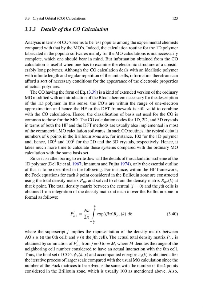
using the total density matrix P μν and solved to obtain the density matrix R μν (k) at
that k point. The total density matrix between the central (j = 0) and the jth cells is
obtained from integration of the density matrix at each k over the Brillouin zone in
formal as follows:
P
j
μν =
Na
2π
π
a
−
π
a
exp[ijka]R μν (k) dk
(3.40)
where the superscript j implies the representation of the density matrix between
AO’s μ (∈ the 0th cell) and ν (∈ the jth cell). The actual total density matrix P μν is
obtained by summation of P
j
μν from j = 0 to ± M, where M denotes the range of the
neighboring cell number considered to have an actual interaction with the 0th cell.
Thus, the final set of CO’s ψ s (k, x) and accompanied energies ε s (k) is obtained after
the iterative process of larger scale compared with the usual MO calculation since the
number of the Fock matrices to be solved is the same with the number of the k points
considered in the Brillouin zone, which is usually 100 as mentioned above. Also,
123
3.3.3 Details of the CO Calculation
Analysis in terms of CO’s seems to be less popular among the experimental chemists
compared with that by the MO’s. Indeed, the calculation routine for the 1D polymer
fabricated in the popular softwares mainly for the MO calculations is not necessarily
complete, which one should bear in mind. But information obtained from the CO
calculation is useful when one has to examine the electronic structure of a considerably long polymer. Although the CO calculation deals with an idealistic polymer
with infinite length and regular repetition of the unit cells, information therefrom can
afford a sort of necessary conditions for the appearance of the electronic properties
of actual polymers.
The CO having the form of Eq. (3.39) is a kind of extended version of the ordinary
MO modified with an introduction of the Bloch theorem necessary for the description
of the 1D polymer. In this sense, the CO’s are within the range of one-electron
approximation and hence the HF or the DFT framework is still valid to combine
with the CO calculation. Hence, the classification of basis set used for the CO is
common to those for the MO. The CO calculation codes for 1D, 2D, and 3D crystals
in terms of both the HF and the DFT methods are usually also implemented in most
of the commercial MO calculation softwares. In such CO routines, the typical default
numbers of k points in the Brillouin zone are, for instance, 100 for the 1D polymer
and, hence, 100
2 and 100
3 for the 2D and the 3D crystals, respectively. Hence, it
takes much more time to calculate these systems compared with the ordinary MO
calculation with the same basis set.
Since it is rather boring to write down all the details of the calculation scheme of the
1D polymer (Del Re et al. 1967; Imamura and Fujita 1974), only the essential outline
of that is to be described in the following. For instance, within the HF framework,
the Fock equations for each k point considered in the Brillouin zone are constructed
using the total density matrix P μν and solved to obtain the density matrix R μν (k) at
that k point. The total density matrix between the central (j = 0) and the jth cells is
obtained from integration of the density matrix at each k over the Brillouin zone in
formal as follows:
P
j
μν =
Na
2π
π
a
−
π
a
exp[ijka]R μν (k) dk
(3.40)
where the superscript j implies the representation of the density matrix between
AO’s μ (∈ the 0th cell) and ν (∈ the jth cell). The actual total density matrix P μν is
obtained by summation of P
j
μν from j = 0 to ± M, where M denotes the range of the
neighboring cell number considered to have an actual interaction with the 0th cell.
Thus, the final set of CO’s ψ s (k, x) and accompanied energies ε s (k) is obtained after
the iterative process of larger scale compared with the usual MO calculation since the
number of the Fock matrices to be solved is the same with the number of the k points
considered in the Brillouin zone, which is usually 100 as mentioned above. Also,