

3.2 Density Functional Theory (DFT) Calculations
115
is proportional to N
3 for the KS equation to solve, whereas N
4 for the HF equation
with N standing for the number of electrons.
Since the KS operator itself contains the electron density derived from the KS
orbitals as in Eq. (3.22), the KS equation has to be iteratively solved starting from
a certain assumption of the initial set of the KS orbitals until obtaining the SCF
solution, i.e., the ‘stable’ set of KS orbitals as in the UHF equation, since the KS
orbitals distinguish the α and β the spins. In order to represent the KS orbitals are
mostly employed the Gauss-type orbitals as the basis sets like in the HF MO’s.
E XC [ρ(r)] and V XC (r) normally contain arithmetically complicated functions and
hence require numerical integrations, for which the sample points called grids are
generated in a precise manner around each atomic nucleus constructing the molecule
to be examined. This allows us to calculate the precise total energy as well as the
energy gradient.
It is of main importance to properly estimate the exchange-correlation potential
V XC (r) or, in other words, exchange-correlation functional of good quality. This
comes from that the results out of the KS equation are determined by the adaptability
and the range of application of the exchange-correlation functional. Unfortunately,
no systematic ways have been manipulated to enhance the approximation level of the
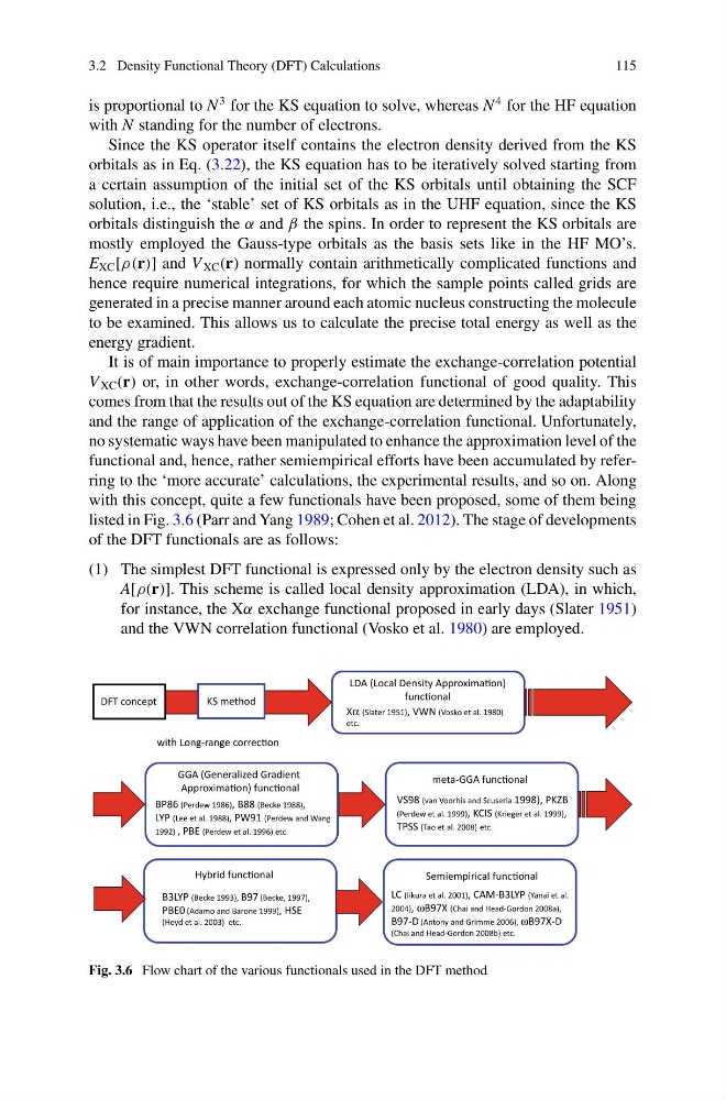
functional and, hence, rather semiempirical efforts have been accumulated by referring to the ‘more accurate’ calculations, the experimental results, and so on. Along
with this concept, quite a few functionals have been proposed, some of them being
listed in Fig. 3.6 (Parr and Yang 1989; Cohen et al. 2012). The stage of developments
of the DFT functionals are as follows:
(1) The simplest DFT functional is expressed only by the electron density such as
A[ρ(r)]. This scheme is called local density approximation (LDA), in which,
for instance, the Xα exchange functional proposed in early days (Slater 1951)
and the VWN correlation functional (Vosko et al. 1980) are employed.
LDA (Local Density ApproximaƟon)
funcƟonal
Xα (Slater 1951), VWN (Vosko et al. 1980)
etc.
KS method
DFT concept
meta-GGA funcƟonal
VS98 (van Voorhis and Scuseria 1998), PKZB
(Perdew et al. 1999), KCIS (Krieger et al. 1999),
TPSS (Tao et al. 2008) etc.
GGA (Generalized Gradient
ApproximaƟon) funcƟonal
BP86 (Perdew 1986), B88 (Becke 1988),
LYP (Lee et al. 1988), PW91 (Perdew and Wang
1992) , PBE (Perdew et al. 1996) etc.
Semiempirical funcƟonal
Hybrid funcƟonal
B3LYP (Becke 1993), B97 (Becke, 1997),
PBE0 (Adamo and Barone 1999), HSE
(Heyd et al. 2003) etc.
LC (Iikura et al. 2001), CAM-B3LYP (Yanai et al.
2004), ωB97X (Chai and Head-Gordon 2008a),
B97-D (Antony and Grimme 2006), ωB97X-D
(Chai and Head-Gordon 2008b) etc.
with Long-range correcƟon
Fig. 3.6 Flow chart of the various functionals used in the DFT method
115
is proportional to N
3 for the KS equation to solve, whereas N
4 for the HF equation
with N standing for the number of electrons.
Since the KS operator itself contains the electron density derived from the KS
orbitals as in Eq. (3.22), the KS equation has to be iteratively solved starting from
a certain assumption of the initial set of the KS orbitals until obtaining the SCF
solution, i.e., the ‘stable’ set of KS orbitals as in the UHF equation, since the KS
orbitals distinguish the α and β the spins. In order to represent the KS orbitals are
mostly employed the Gauss-type orbitals as the basis sets like in the HF MO’s.
E XC [ρ(r)] and V XC (r) normally contain arithmetically complicated functions and
hence require numerical integrations, for which the sample points called grids are
generated in a precise manner around each atomic nucleus constructing the molecule
to be examined. This allows us to calculate the precise total energy as well as the
energy gradient.
It is of main importance to properly estimate the exchange-correlation potential
V XC (r) or, in other words, exchange-correlation functional of good quality. This
comes from that the results out of the KS equation are determined by the adaptability
and the range of application of the exchange-correlation functional. Unfortunately,
no systematic ways have been manipulated to enhance the approximation level of the
functional and, hence, rather semiempirical efforts have been accumulated by referring to the ‘more accurate’ calculations, the experimental results, and so on. Along
with this concept, quite a few functionals have been proposed, some of them being
listed in Fig. 3.6 (Parr and Yang 1989; Cohen et al. 2012). The stage of developments
of the DFT functionals are as follows:
(1) The simplest DFT functional is expressed only by the electron density such as
A[ρ(r)]. This scheme is called local density approximation (LDA), in which,
for instance, the Xα exchange functional proposed in early days (Slater 1951)
and the VWN correlation functional (Vosko et al. 1980) are employed.
LDA (Local Density ApproximaƟon)
funcƟonal
Xα (Slater 1951), VWN (Vosko et al. 1980)
etc.
KS method
DFT concept
meta-GGA funcƟonal
VS98 (van Voorhis and Scuseria 1998), PKZB
(Perdew et al. 1999), KCIS (Krieger et al. 1999),
TPSS (Tao et al. 2008) etc.
GGA (Generalized Gradient
ApproximaƟon) funcƟonal
BP86 (Perdew 1986), B88 (Becke 1988),
LYP (Lee et al. 1988), PW91 (Perdew and Wang
1992) , PBE (Perdew et al. 1996) etc.
Semiempirical funcƟonal
Hybrid funcƟonal
B3LYP (Becke 1993), B97 (Becke, 1997),
PBE0 (Adamo and Barone 1999), HSE
(Heyd et al. 2003) etc.
LC (Iikura et al. 2001), CAM-B3LYP (Yanai et al.
2004), ωB97X (Chai and Head-Gordon 2008a),
B97-D (Antony and Grimme 2006), ωB97X-D
(Chai and Head-Gordon 2008b) etc.
with Long-range correcƟon
Fig. 3.6 Flow chart of the various functionals used in the DFT method