

13 Study of Formalization of Informal Collectors …
181
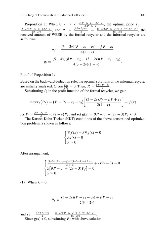
Proposition 1: When 0 < v <
3(P−c 1 −c 2 )−β P+c 1
2(P−c 1 −c 2 )
, the optimal price P f =
(3−2v)(P−c1−c2)+β P−c 1
2(3−2v)
, and P i =
β P+P f −c 1
2
=
(3−2v)(P−c1−c2)+(7−4v)(β P−c 1 )
4(3−2v)
, the
received amount of WEEE by the formal recycler and the informal recycler are
as follows:
q f =
(3 − 2v)(P − c 1 − c 2 ) − β P + c 1
4(1 − v)
q i =
(5 − 4v)(β P − c 1 ) − (3 − 2v)(P − c 1 − c 2 )
4(3 − 2v)(1 − v)
.
Proof of Proposition 1:
Based on the backward deduction rule, the optimal solutions of the informal recycler
are initially analyzed. Given
∂π i
∂ P i
= 0, Then, P i =
β P+P f −c 1
2
.
Substituting P i in the profit function of the formal recycler, we gain:
maxπ f
P f
=
P − P f − c 1 − c 2
(3 − 2v)P f − β P + c 1
2(1 − v)
= f (x)
s.t.P i =
β P+P f −c 1
2
< (2 − v)P f , and set g(x) = β P − c 1 + (2v − 3)P f < 0.
The Karush-Kuhn-Tucker (KKT) conditions of the above constrained optimization problem is shown as follows:
⎧
⎨
⎩
∇ f (x) + λ∇g(x) = 0
λg(x) = 0
λ ≥ 0
After arrangement,
⎧
⎪ ⎨
⎪ ⎩
(3−2v)(P−c1−c2)−2(3−2v)Pf +β P−c 1
2(1−v)
+ λ(2v − 3) = 0
λ
β P − c 1 + (2v − 3)P f
= 0
λ ≥ 0
,
(1) When λ = 0,
P f =
(3 − 2v)(P − c 1 − c 2 ) + β P − c 1
2(3 − 2v)
,
and P i =
β P+P f −c 1
2
=
(3−2v)(P−c1−c2)+(7−4v)(β P−c 1 )
4(3−2v)
.
Since g(x) < 0, substituting P f with above solution,
181
Proposition 1: When 0 < v <
3(P−c 1 −c 2 )−β P+c 1
2(P−c 1 −c 2 )
, the optimal price P f =
(3−2v)(P−c1−c2)+β P−c 1
2(3−2v)
, and P i =
β P+P f −c 1
2
=
(3−2v)(P−c1−c2)+(7−4v)(β P−c 1 )
4(3−2v)
, the
received amount of WEEE by the formal recycler and the informal recycler are
as follows:
q f =
(3 − 2v)(P − c 1 − c 2 ) − β P + c 1
4(1 − v)
q i =
(5 − 4v)(β P − c 1 ) − (3 − 2v)(P − c 1 − c 2 )
4(3 − 2v)(1 − v)
.
Proof of Proposition 1:
Based on the backward deduction rule, the optimal solutions of the informal recycler
are initially analyzed. Given
∂π i
∂ P i
= 0, Then, P i =
β P+P f −c 1
2
.
Substituting P i in the profit function of the formal recycler, we gain:
maxπ f
P f
=
P − P f − c 1 − c 2
(3 − 2v)P f − β P + c 1
2(1 − v)
= f (x)
s.t.P i =
β P+P f −c 1
2
< (2 − v)P f , and set g(x) = β P − c 1 + (2v − 3)P f < 0.
The Karush-Kuhn-Tucker (KKT) conditions of the above constrained optimization problem is shown as follows:
⎧
⎨
⎩
∇ f (x) + λ∇g(x) = 0
λg(x) = 0
λ ≥ 0
After arrangement,
⎧
⎪ ⎨
⎪ ⎩
(3−2v)(P−c1−c2)−2(3−2v)Pf +β P−c 1
2(1−v)
+ λ(2v − 3) = 0
λ
β P − c 1 + (2v − 3)P f
= 0
λ ≥ 0
,
(1) When λ = 0,
P f =
(3 − 2v)(P − c 1 − c 2 ) + β P − c 1
2(3 − 2v)
,
and P i =
β P+P f −c 1
2
=
(3−2v)(P−c1−c2)+(7−4v)(β P−c 1 )
4(3−2v)
.
Since g(x) < 0, substituting P f with above solution,