

quantitative differences between laboratory animal species and humans in the disposition of
inhaled ozone which minimize the utility of the
data from laboratory animals for quantitatively
estimating human risk of ozone exposures.
The effects of ozone on the respiratory tract are
well known, thus it is not surprising that consideration of these effects has had a primary influence
on the setting of the Ozone NAAQS. In the review
culminating with a revised standard in March
2008, the information from pulmonary function
evaluations conducted on young adult volunteers
undergoing moderate exercise while exposed to
various concentrations of ozone for 6.6 h played a
prominent role. The key parameter evaluated,
changes in the forced expiratory volume in 1 s
(FEV 1 ), are shown in Fig. 10 [1–3, 13, 24, 26, 44,
45]. Data from individuals exposed to 0.08 ppm
ozone and higher were considered in the previous
review of the ozone standard. In the most recent
review, data were available from the studies of
Adams and colleagues [3] with 0.06 and
0.04 ppm exposures conducted to complement
earlier studies conducted with 0.08 and
0.012 ppm, Adams [3] interpreted his studies as
showing a statistically significant effect at
0.08 ppm, effectively reproducing the effects
seen in earlier studies. However, he interpreted
his studies at 0.06 and 0.04 ppm as not showing
statistically significant changes compared to
exposure to clean air. The USEPA reanalyzed the
data of Adams and colleagues using different statistical procedures [13]. The USEPA reanalysis
was included in the final compilation of information provided to the EPA Administrator to render a
judgment on the revision of the Ozone NAAQS.
A key piece of information on the health effects
of ozone came from the time-series study of Bell
et al. [8, 9]. Their analysis used a 24-h averaging
time and, thus, was not directly applicable to
setting the Ozone NAAQS with an 8-h averaging
time. Smith et al. [58] extended the analyses of
Bell et al. [8] focusing on the development of cityspecific ozone mortality estimates. The analyses
of both Bell et al. [8] and Smith et al. [58] used the
National Air Pollution Morbidity and Mortality
air pollution database assembled at Johns Hopkins
University. The results for the 8-h averaging time
are shown in Fig. 11. The degree of intercity
heterogeneity is noteworthy including recognition
that only 5 cities of the 98 cities evaluated had
statistically significant effects of ozone on acute
mortality.
Smith et al. [58] called attention to this
intercity heterogeneity across the United States
(Fig. 12). The ozone effects are most striking in
the Northeastern United States and absent in the
Western United States including the Los Angeles
Basin. It is not surprising that Smith et al. [58]
caution against the use of national estimates of
ozone concentration-response functions.
The EPA’s CASAC recommended to the
Administrator that he revise the Ozone NAAQS
with an 8-h averaging time, from 0.08 ppm to a
level within the range of 0.060–0.070 ppm. Ultimately, the Administrator exercised his judgment
0
0.00
ppb
−1
0.01
0.02
0.03
0.04
0.05
20
Ozone (ppb)
40
60
80
100
Air
Quality
Guidelines
and
Standards,
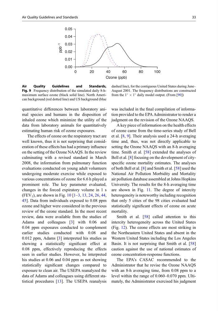
Fig. 9 Frequency distribution of the simulated daily 8-hmaximum surface ozone (black solid line). North American background (red dotted line) and US background (blue
dashed line), for the contiguous United States during June–
August 2001. The frequency distributions are constructed
from the 1
 1
daily model output. (From [90])
Air Quality Guidelines and Standards
33
inhaled ozone which minimize the utility of the
data from laboratory animals for quantitatively
estimating human risk of ozone exposures.
The effects of ozone on the respiratory tract are
well known, thus it is not surprising that consideration of these effects has had a primary influence
on the setting of the Ozone NAAQS. In the review
culminating with a revised standard in March
2008, the information from pulmonary function
evaluations conducted on young adult volunteers
undergoing moderate exercise while exposed to
various concentrations of ozone for 6.6 h played a
prominent role. The key parameter evaluated,
changes in the forced expiratory volume in 1 s
(FEV 1 ), are shown in Fig. 10 [1–3, 13, 24, 26, 44,
45]. Data from individuals exposed to 0.08 ppm
ozone and higher were considered in the previous
review of the ozone standard. In the most recent
review, data were available from the studies of
Adams and colleagues [3] with 0.06 and
0.04 ppm exposures conducted to complement
earlier studies conducted with 0.08 and
0.012 ppm, Adams [3] interpreted his studies as
showing a statistically significant effect at
0.08 ppm, effectively reproducing the effects
seen in earlier studies. However, he interpreted
his studies at 0.06 and 0.04 ppm as not showing
statistically significant changes compared to
exposure to clean air. The USEPA reanalyzed the
data of Adams and colleagues using different statistical procedures [13]. The USEPA reanalysis
was included in the final compilation of information provided to the EPA Administrator to render a
judgment on the revision of the Ozone NAAQS.
A key piece of information on the health effects
of ozone came from the time-series study of Bell
et al. [8, 9]. Their analysis used a 24-h averaging
time and, thus, was not directly applicable to
setting the Ozone NAAQS with an 8-h averaging
time. Smith et al. [58] extended the analyses of
Bell et al. [8] focusing on the development of cityspecific ozone mortality estimates. The analyses
of both Bell et al. [8] and Smith et al. [58] used the
National Air Pollution Morbidity and Mortality
air pollution database assembled at Johns Hopkins
University. The results for the 8-h averaging time
are shown in Fig. 11. The degree of intercity
heterogeneity is noteworthy including recognition
that only 5 cities of the 98 cities evaluated had
statistically significant effects of ozone on acute
mortality.
Smith et al. [58] called attention to this
intercity heterogeneity across the United States
(Fig. 12). The ozone effects are most striking in
the Northeastern United States and absent in the
Western United States including the Los Angeles
Basin. It is not surprising that Smith et al. [58]
caution against the use of national estimates of
ozone concentration-response functions.
The EPA’s CASAC recommended to the
Administrator that he revise the Ozone NAAQS
with an 8-h averaging time, from 0.08 ppm to a
level within the range of 0.060–0.070 ppm. Ultimately, the Administrator exercised his judgment
0
0.00
ppb
−1
0.01
0.02
0.03
0.04
0.05
20
Ozone (ppb)
40
60
80
100
Air
Quality
Guidelines
and
Standards,
Fig. 9 Frequency distribution of the simulated daily 8-hmaximum surface ozone (black solid line). North American background (red dotted line) and US background (blue
dashed line), for the contiguous United States during June–
August 2001. The frequency distributions are constructed
from the 1
 1
daily model output. (From [90])
Air Quality Guidelines and Standards
33