

50 unifying physics of accelerators, lasers and plasma
where the parenthesis with Twiss functions in front of the numerical coefficient is usually called H. As we see, the back-ofthe-envelope estimation correctly captures the most important features of the phenomenon and also produces a useful
and simple expression.
3.2.3 Equilibrium emittance
The SR-induced cooling of the beam emittance and SRinduced emittance growth would naturally balance, so that
the beam emittance would eventually reach equilibrium
value.
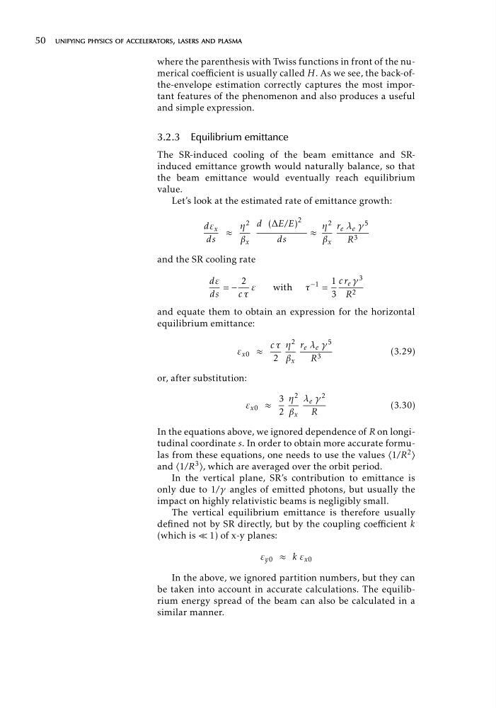
Let’s look at the estimated rate of emittance growth:
2
η 2
dε
d (ΔE/E)
x
η 2 r λ γ 5
ds
≈ β
≈
e e
x
ds
β x
R 3
and the SR cooling rate
3
dε
2
1 c r γ
= − ε
with
−1
e
τ =
ds
c τ
3 R 2
and equate them to obtain an expression for the horizontal
equilibrium emittance:
c τ η 2 r
5
e λ e γ
ε x0 ≈
(3.29)
2 β
R 3
x
or, after substitution:
3 η 2 λ
ε x0 ≈
e γ 2
(3.30)
2 β x R
In the equations above, we ignored dependence of R on longitudinal coordinate s. In order to obtain more accurate formulas from these equations, one needs to use the values 1/R 2
and (1/R 3 ), which are averaged over the orbit period.
(
)
In the vertical plane, SR’s contribution to emittance is
only due to 1/γ angles of emitted photons, but usually the
impact on highly relativistic beams is negligibly small.
The vertical equilibrium emittance is therefore usually
defined not by SR directly, but by the coupling coefficient k
(which is « 1) of x-y planes:
ε y0 ≈ k ε x0
In the above, we ignored partition numbers, but they can
be taken into account in accurate calculations. The equilibrium energy spread of the beam can also be calculated in a
similar manner.
where the parenthesis with Twiss functions in front of the numerical coefficient is usually called H. As we see, the back-ofthe-envelope estimation correctly captures the most important features of the phenomenon and also produces a useful
and simple expression.
3.2.3 Equilibrium emittance
The SR-induced cooling of the beam emittance and SRinduced emittance growth would naturally balance, so that
the beam emittance would eventually reach equilibrium
value.
Let’s look at the estimated rate of emittance growth:
2
η 2
dε
d (ΔE/E)
x
η 2 r λ γ 5
ds
≈ β
≈
e e
x
ds
β x
R 3
and the SR cooling rate
3
dε
2
1 c r γ
= − ε
with
−1
e
τ =
ds
c τ
3 R 2
and equate them to obtain an expression for the horizontal
equilibrium emittance:
c τ η 2 r
5
e λ e γ
ε x0 ≈
(3.29)
2 β
R 3
x
or, after substitution:
3 η 2 λ
ε x0 ≈
e γ 2
(3.30)
2 β x R
In the equations above, we ignored dependence of R on longitudinal coordinate s. In order to obtain more accurate formulas from these equations, one needs to use the values 1/R 2
and (1/R 3 ), which are averaged over the orbit period.
(
)
In the vertical plane, SR’s contribution to emittance is
only due to 1/γ angles of emitted photons, but usually the
impact on highly relativistic beams is negligibly small.
The vertical equilibrium emittance is therefore usually
defined not by SR directly, but by the coupling coefficient k
(which is « 1) of x-y planes:
ε y0 ≈ k ε x0
In the above, we ignored partition numbers, but they can
be taken into account in accurate calculations. The equilibrium energy spread of the beam can also be calculated in a
similar manner.