

86 unifying physics of accelerators, lasers and plasma
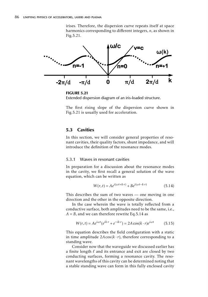
irises. Therefore, the dispersion curve repeats itself at space
harmonics corresponding to different integers, n, as shown in
Fig.5.21.
F
N
N
FIGURE 5.21
Extended dispersion diagram of an iris-loaded structure.
The first rising slope of the dispersion curve shown in
Fig.5.21 is usually used for acceleration.
5.3 Cavities
In this section, we will consider general properties of resonant cavities, their quality factors, shunt impedance, and will
introduce the definition of the resonance modes.
5.3.1 Waves in resonant cavities
In preparation for a discussion about the resonance modes
in the cavity, we first recall a general solution of the wave
equation, which can be written as
W (r, t) = Ae
i(ωt+k·r) + Be
i(ωt−k·r)
(5.14)
This describes the sum of two waves — one moving in one
direction and the other in the opposite direction.
In the case wherein the wave is totally reflected from a
conductive surface, both amplitudes need to be the same, i.e.,
A = B, and we can therefore rewrite Eq.5.14 as
ik·r + e
iωt
W (r, t) = Ae
iωt (e
−ik·r ) = 2A cos(k · r)e
(5.15)
This equation describes the field configuration with a static
in time amplitude 2A cos (k · r), therefore corresponding to a
standing wave.
Consider now that the waveguide we discussed earlier has
a finite length e and its entrance and exit are closed by two
conducting surfaces, forming a resonance cavity. The resonant wavelengths of this cavity can be determined noting that
a stable standing wave can form in this fully enclosed cavity
irises. Therefore, the dispersion curve repeats itself at space
harmonics corresponding to different integers, n, as shown in
Fig.5.21.
F
N
N
FIGURE 5.21
Extended dispersion diagram of an iris-loaded structure.
The first rising slope of the dispersion curve shown in
Fig.5.21 is usually used for acceleration.
5.3 Cavities
In this section, we will consider general properties of resonant cavities, their quality factors, shunt impedance, and will
introduce the definition of the resonance modes.
5.3.1 Waves in resonant cavities
In preparation for a discussion about the resonance modes
in the cavity, we first recall a general solution of the wave
equation, which can be written as
W (r, t) = Ae
i(ωt+k·r) + Be
i(ωt−k·r)
(5.14)
This describes the sum of two waves — one moving in one
direction and the other in the opposite direction.
In the case wherein the wave is totally reflected from a
conductive surface, both amplitudes need to be the same, i.e.,
A = B, and we can therefore rewrite Eq.5.14 as
ik·r + e
iωt
W (r, t) = Ae
iωt (e
−ik·r ) = 2A cos(k · r)e
(5.15)
This equation describes the field configuration with a static
in time amplitude 2A cos (k · r), therefore corresponding to a
standing wave.
Consider now that the waveguide we discussed earlier has
a finite length e and its entrance and exit are closed by two
conducting surfaces, forming a resonance cavity. The resonant wavelengths of this cavity can be determined noting that
a stable standing wave can form in this fully enclosed cavity