

82
An Introduction to Beam Physics
[
ZHDNHUILHOG
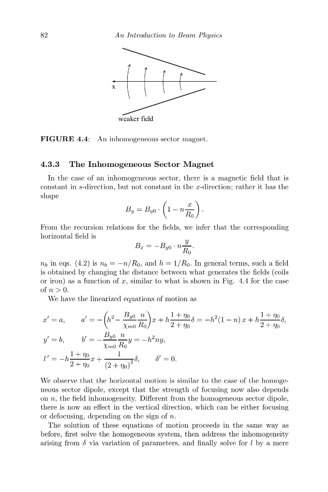
FIGURE 4.4: An inhomogeneous sector magnet.
4.3.3 The Inhomogeneous Sector Magnet
In the case of an inhomogeneous sector, there is a magnetic field that is
constant in s-direction, but not constant in the x-direction; rather it has the
shape
B y = B y0 ·
1 − n
x
R 0
.
From the recursion relations for the fields, we infer that the corresponding
horizontal field is
B x = −B y0 · n
y
R 0
.
n b in eqs. (4.2) is n b = −n/R 0 , and h = 1/R 0 . In general terms, such a field
is obtained by changing the distance between what generates the fields (coils
or iron) as a function of x, similar to what is shown in Fig. 4.4 for the case
of n > 0.
We have the linearized equations of motion as
x
= a,
a
= −
h
2
−
B y0
χ m0
n
R 0
x + h
1 + η 0
2 + η 0
δ = −h
2 (1 − n) x + h
1 + η 0
2 + η 0
δ,
y
= b,
b
= −
B y0
χ m0
n
R 0
y = −h
2 ny,
l
= −h
1 + η 0
2 + η 0
x +
1
(2 + η 0 )
2 δ,
δ
= 0.
We observe that the horizontal motion is similar to the case of the homogeneous sector dipole, except that the strength of focusing now also depends
on n, the field inhomogeneity. Different from the homogeneous sector dipole,
there is now an effect in the vertical direction, which can be either focusing
or defocusing, depending on the sign of n.
The solution of these equations of motion proceeds in the same way as
before, first solve the homogeneous system, then address the inhomogeneity
arising from δ via variation of parameters, and finally solve for l by a mere
An Introduction to Beam Physics
[
ZHDNHUILHOG
FIGURE 4.4: An inhomogeneous sector magnet.
4.3.3 The Inhomogeneous Sector Magnet
In the case of an inhomogeneous sector, there is a magnetic field that is
constant in s-direction, but not constant in the x-direction; rather it has the
shape
B y = B y0 ·
1 − n
x
R 0
.
From the recursion relations for the fields, we infer that the corresponding
horizontal field is
B x = −B y0 · n
y
R 0
.
n b in eqs. (4.2) is n b = −n/R 0 , and h = 1/R 0 . In general terms, such a field
is obtained by changing the distance between what generates the fields (coils
or iron) as a function of x, similar to what is shown in Fig. 4.4 for the case
of n > 0.
We have the linearized equations of motion as
x
= a,
a
= −
h
2
−
B y0
χ m0
n
R 0
x + h
1 + η 0
2 + η 0
δ = −h
2 (1 − n) x + h
1 + η 0
2 + η 0
δ,
y
= b,
b
= −
B y0
χ m0
n
R 0
y = −h
2 ny,
l
= −h
1 + η 0
2 + η 0
x +
1
(2 + η 0 )
2 δ,
δ
= 0.
We observe that the horizontal motion is similar to the case of the homogeneous sector dipole, except that the strength of focusing now also depends
on n, the field inhomogeneity. Different from the homogeneous sector dipole,
there is now an effect in the vertical direction, which can be either focusing
or defocusing, depending on the sign of n.
The solution of these equations of motion proceeds in the same way as
before, first solve the homogeneous system, then address the inhomogeneity
arising from δ via variation of parameters, and finally solve for l by a mere