

72
An Introduction to Beam Physics
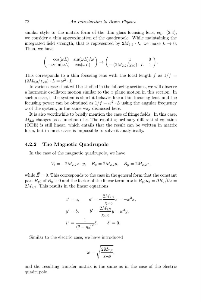
similar style to the matrix form of the thin glass focusing lens, eq. (2.4),
we consider a thin approximation of the quadrupole. While maintaining the
integrated field strength, that is represented by 2M 2,2 · L, we make L → 0.
Then, we have
cos(ωL) sin(ωL)/ω
−ω sin(ωL) cos(ωL)
→
1
0
− (2M 2,2 /χ e0 ) · L 1
.
This corresponds to a thin focusing lens with the focal length f as 1/f =
(2M 2,2 /χ e0 ) · L = ω
2
· L.
In various cases that will be studied in the following sections, we will observe
a harmonic oscillator motion similar to the x plane motion in this section. In
such a case, if the system is short it behaves like a thin focusing lens, and the
focusing power can be obtained as 1/f = ω
2
· L using the angular frequency
ω of the system, in the same way discussed here.
It is also worthwhile to briefly mention the case of fringe fields. In this case,
M 2,2 changes as a function of s. The resulting ordinary differential equation
(ODE) is still linear, which entails that the result can be written in matrix
form, but in most cases is impossible to solve it analytically.
4.2.2 The Magnetic Quadrupole
In the case of the magnetic quadrupole, we have
V b = −2M 2,2 x · y, B x = 2M 2,2 y, B y = 2M 2,2 x,
while
E = 0. This corresponds to the case in the general form that the constant
part B y0 of B y is 0 and the factor of the linear term in x is B y0 n b = ∂B y /∂x =
2M 2,2 . This results in the linear equations
x
= a,
a
= −
2M 2,2
χ m0
x = −ω
2 x,
y
= b,
b
=
2M 2,2
χ m0
y = ω
2 y,
l
=
1
(2 + η 0 )
2 δ,
δ
= 0.
Similar to the electric case, we have introduced
ω =
2M 2,2
χ m0
,
and the resulting transfer matrix is the same as in the case of the electric
quadrupole.
An Introduction to Beam Physics
similar style to the matrix form of the thin glass focusing lens, eq. (2.4),
we consider a thin approximation of the quadrupole. While maintaining the
integrated field strength, that is represented by 2M 2,2 · L, we make L → 0.
Then, we have
cos(ωL) sin(ωL)/ω
−ω sin(ωL) cos(ωL)
→
1
0
− (2M 2,2 /χ e0 ) · L 1
.
This corresponds to a thin focusing lens with the focal length f as 1/f =
(2M 2,2 /χ e0 ) · L = ω
2
· L.
In various cases that will be studied in the following sections, we will observe
a harmonic oscillator motion similar to the x plane motion in this section. In
such a case, if the system is short it behaves like a thin focusing lens, and the
focusing power can be obtained as 1/f = ω
2
· L using the angular frequency
ω of the system, in the same way discussed here.
It is also worthwhile to briefly mention the case of fringe fields. In this case,
M 2,2 changes as a function of s. The resulting ordinary differential equation
(ODE) is still linear, which entails that the result can be written in matrix
form, but in most cases is impossible to solve it analytically.
4.2.2 The Magnetic Quadrupole
In the case of the magnetic quadrupole, we have
V b = −2M 2,2 x · y, B x = 2M 2,2 y, B y = 2M 2,2 x,
while
E = 0. This corresponds to the case in the general form that the constant
part B y0 of B y is 0 and the factor of the linear term in x is B y0 n b = ∂B y /∂x =
2M 2,2 . This results in the linear equations
x
= a,
a
= −
2M 2,2
χ m0
x = −ω
2 x,
y
= b,
b
=
2M 2,2
χ m0
y = ω
2 y,
l
=
1
(2 + η 0 )
2 δ,
δ
= 0.
Similar to the electric case, we have introduced
ω =
2M 2,2
χ m0
,
and the resulting transfer matrix is the same as in the case of the electric
quadrupole.