

68
An Introduction to Beam Physics
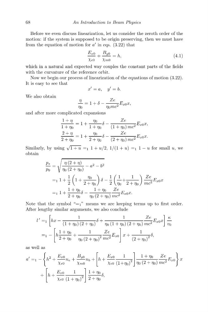
Before we even discuss linearization, let us consider the zeroth order of the
motion: if the system is supposed to be origin preserving, then we must have
from the equation of motion for a
in eqs. (3.22) that
E x0
χ e0
+
B y0
χ m0
= h,
(4.1)
which in a natural and expected way couples the constant parts of the fields
with the curvature of the reference orbit.
Now we begin our process of linearization of the equations of motion (3.22).
It is easy to see that
x
= a, y
= b.
We also obtain
η
η 0
= 1 + δ −
Ze
η 0 mc 2 E x0 x,
and after more complicated expansions
1 + η
1 + η 0
= 1 +
η 0
1 + η 0
δ −
Ze
(1 + η 0 ) mc 2 E x0 x,
2 + η
2 + η 0
= 1 +
η 0
2 + η 0
δ −
Ze
(2 + η 0 ) mc 2 E x0 x.
Similarly, by using
√
1 + u = 1 1 + u/2, 1/(1 + u) = 1 1 − u for small u, we
obtain
p s
p 0
=
η (2 + η)
η 0 (2 + η 0 )
− a 2 − b 2
= 1 1 +
1
2
1 +
η 0
2 + η 0
δ −
1
2
1
η 0
+
1
2 + η 0
Ze
mc 2 E x0 x
= 1 1 +
1 + η 0
2 + η 0
δ −
1 + η 0
η 0 (2 + η 0 )
Ze
mc 2 E x0 x.
Note that the symbol “= 1 ” means we are keeping terms up to first order.
After lengthy similar arguments, we also conclude
l
= 1
hx −
1
(1 + η 0 ) (2 + η 0 )
δ +
1
η 0 (1 + η 0 ) (2 + η 0 )
Ze
mc 2 E x0 x
κ
v 0
= 1 −
h
1 + η 0
2 + η 0
+
1
η 0 (2 + η 0 )
2
Ze
mc 2 E x0
x +
1
(2 + η 0 )
2 δ,
as well as
a
= 1 −
h
2 +
E x0
χ e0
n e +
B y0
χ m0
n b +
h +
E x0
χ e0
1
(1+η 0 )
2
1 + η 0
η 0 (2 + η 0 )
Ze
mc 2 E x0
x
+
h +
E x0
χ e0
1
(1 + η 0 )
2
1 + η 0
2 + η 0
δ,
An Introduction to Beam Physics
Before we even discuss linearization, let us consider the zeroth order of the
motion: if the system is supposed to be origin preserving, then we must have
from the equation of motion for a
in eqs. (3.22) that
E x0
χ e0
+
B y0
χ m0
= h,
(4.1)
which in a natural and expected way couples the constant parts of the fields
with the curvature of the reference orbit.
Now we begin our process of linearization of the equations of motion (3.22).
It is easy to see that
x
= a, y
= b.
We also obtain
η
η 0
= 1 + δ −
Ze
η 0 mc 2 E x0 x,
and after more complicated expansions
1 + η
1 + η 0
= 1 +
η 0
1 + η 0
δ −
Ze
(1 + η 0 ) mc 2 E x0 x,
2 + η
2 + η 0
= 1 +
η 0
2 + η 0
δ −
Ze
(2 + η 0 ) mc 2 E x0 x.
Similarly, by using
√
1 + u = 1 1 + u/2, 1/(1 + u) = 1 1 − u for small u, we
obtain
p s
p 0
=
η (2 + η)
η 0 (2 + η 0 )
− a 2 − b 2
= 1 1 +
1
2
1 +
η 0
2 + η 0
δ −
1
2
1
η 0
+
1
2 + η 0
Ze
mc 2 E x0 x
= 1 1 +
1 + η 0
2 + η 0
δ −
1 + η 0
η 0 (2 + η 0 )
Ze
mc 2 E x0 x.
Note that the symbol “= 1 ” means we are keeping terms up to first order.
After lengthy similar arguments, we also conclude
l
= 1
hx −
1
(1 + η 0 ) (2 + η 0 )
δ +
1
η 0 (1 + η 0 ) (2 + η 0 )
Ze
mc 2 E x0 x
κ
v 0
= 1 −
h
1 + η 0
2 + η 0
+
1
η 0 (2 + η 0 )
2
Ze
mc 2 E x0
x +
1
(2 + η 0 )
2 δ,
as well as
a
= 1 −
h
2 +
E x0
χ e0
n e +
B y0
χ m0
n b +
h +
E x0
χ e0
1
(1+η 0 )
2
1 + η 0
η 0 (2 + η 0 )
Ze
mc 2 E x0
x
+
h +
E x0
χ e0
1
(1 + η 0 )
2
1 + η 0
2 + η 0
δ,