

58
An Introduction to Beam Physics
the following way:
z ↔ y,
r ↔ (1 + hx) · R(s),
φ ↔
s
R(s)
.
As we recall, in cylindrical coordinates the Laplacian had the form
ΔV (r, φ, z) =
1
r
∂
∂r
r
∂V
∂r
+
1
r
∂
∂φ
1
r
∂V
∂φ
+
∂
2 V
∂z 2 .
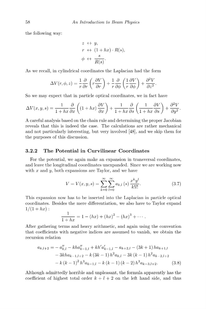
So we may expect that in particle optical coordinates, we in fact have
ΔV (x, y, s) =
1
1 + hx
∂
∂x
(1 + hx)
∂V
∂x
+
1
1 + hx
∂
∂s
1
1 + hx
∂V
∂s
+
∂
2 V
∂y 2 .
A careful analysis based on the chain rule and determining the proper Jacobian
reveals that this is indeed the case. The calculations are rather mechanical
and not particularly interesting, but very involved [48], and we skip them for
the purposes of this discussion.
3.2.2 The Potential in Curvilinear Coordinates
For the potential, we again make an expansion in transversal coordinates,
and leave the longitudinal coordinates unexpanded. Since we are working now
with x and y, both expansions are Taylor, and we have
V = V (x, y, s) =
∞
k=0
∞
l=0
a k,l (s)
x
k y
l
k!l!
.
(3.7)
This expansion now has to be inserted into the Laplacian in particle optical
coordinates. Besides the mere differentiation, we also have to Taylor expand
1/(1 + hx) :
1
1 + hx
= 1 − (hx) + (hx)
2 − (hx)
3 + · · · .
After gathering terms and heavy arithmetic, and again using the convention
that coefficients with negative indices are assumed to vanish, we obtain the
recursion relation
a k,l+2 = − a
k,l − kha
k−1,l + kh
a
k−1,l − a k+2,l − (3k + 1) ha k+1,l
− 3kha k−1,l+2 − k (3k − 1) h
2 a k,l − 3k (k − 1) h
2 a k−2,l+2
− k (k − 1)
2 h
3 a k−1,l − k (k − 1) (k − 2) h
3 a k−3,l+2 .
(3.8)
Although admittedly horrible and unpleasant, the formula apparently has the
coefficient of highest total order k + l + 2 on the left hand side, and thus
An Introduction to Beam Physics
the following way:
z ↔ y,
r ↔ (1 + hx) · R(s),
φ ↔
s
R(s)
.
As we recall, in cylindrical coordinates the Laplacian had the form
ΔV (r, φ, z) =
1
r
∂
∂r
r
∂V
∂r
+
1
r
∂
∂φ
1
r
∂V
∂φ
+
∂
2 V
∂z 2 .
So we may expect that in particle optical coordinates, we in fact have
ΔV (x, y, s) =
1
1 + hx
∂
∂x
(1 + hx)
∂V
∂x
+
1
1 + hx
∂
∂s
1
1 + hx
∂V
∂s
+
∂
2 V
∂y 2 .
A careful analysis based on the chain rule and determining the proper Jacobian
reveals that this is indeed the case. The calculations are rather mechanical
and not particularly interesting, but very involved [48], and we skip them for
the purposes of this discussion.
3.2.2 The Potential in Curvilinear Coordinates
For the potential, we again make an expansion in transversal coordinates,
and leave the longitudinal coordinates unexpanded. Since we are working now
with x and y, both expansions are Taylor, and we have
V = V (x, y, s) =
∞
k=0
∞
l=0
a k,l (s)
x
k y
l
k!l!
.
(3.7)
This expansion now has to be inserted into the Laplacian in particle optical
coordinates. Besides the mere differentiation, we also have to Taylor expand
1/(1 + hx) :
1
1 + hx
= 1 − (hx) + (hx)
2 − (hx)
3 + · · · .
After gathering terms and heavy arithmetic, and again using the convention
that coefficients with negative indices are assumed to vanish, we obtain the
recursion relation
a k,l+2 = − a
k,l − kha
k−1,l + kh
a
k−1,l − a k+2,l − (3k + 1) ha k+1,l
− 3kha k−1,l+2 − k (3k − 1) h
2 a k,l − 3k (k − 1) h
2 a k−2,l+2
− k (k − 1)
2 h
3 a k−1,l − k (k − 1) (k − 2) h
3 a k−3,l+2 .
(3.8)
Although admittedly horrible and unpleasant, the formula apparently has the
coefficient of highest total order k + l + 2 on the left hand side, and thus