

54
An Introduction to Beam Physics
x
y
−
−
+
+
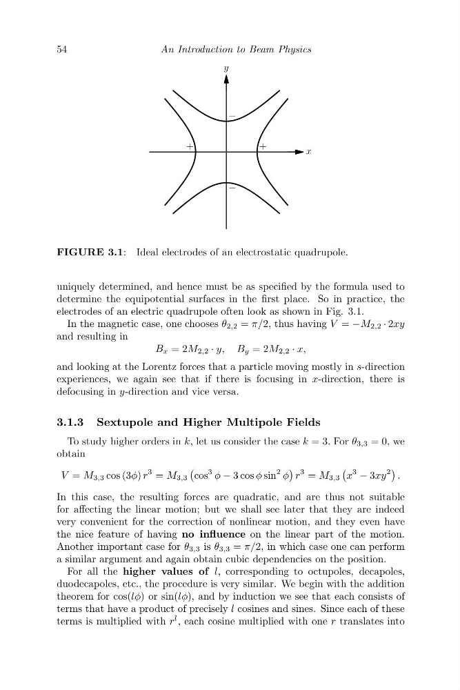
FIGURE 3.1: Ideal electrodes of an electrostatic quadrupole.
uniquely determined, and hence must be as specified by the formula used to
determine the equipotential surfaces in the first place. So in practice, the
electrodes of an electric quadrupole often look as shown in Fig. 3.1.
In the magnetic case, one chooses θ 2,2 = π/2, thus having V = −M 2,2 · 2xy
and resulting in
B x = 2M 2,2 · y, B y = 2M 2,2 · x,
and looking at the Lorentz forces that a particle moving mostly in s-direction
experiences, we again see that if there is focusing in x-direction, there is
defocusing in y-direction and vice versa.
3.1.3 Sextupole and Higher Multipole Fields
To study higher orders in k, let us consider the case k = 3. For θ 3,3 = 0, we
obtain
V = M 3,3 cos (3φ) r
3 = M 3,3
cos
3 φ − 3 cos φ sin
2 φ
r
3 = M 3,3
x
3
− 3xy
2
.
In this case, the resulting forces are quadratic, and are thus not suitable
for affecting the linear motion; but we shall see later that they are indeed
very convenient for the correction of nonlinear motion, and they even have
the nice feature of having no influence on the linear part of the motion.
Another important case for θ 3,3 is θ 3,3 = π/2, in which case one can perform
a similar argument and again obtain cubic dependencies on the position.
For all the higher values of l, corresponding to octupoles, decapoles,
duodecapoles, etc., the procedure is very similar. We begin with the addition
theorem for cos(lφ) or sin(lφ), and by induction we see that each consists of
terms that have a product of precisely l cosines and sines. Since each of these
terms is multiplied with r
l , each cosine multiplied with one r translates into
An Introduction to Beam Physics
x
y
−
−
+
+
FIGURE 3.1: Ideal electrodes of an electrostatic quadrupole.
uniquely determined, and hence must be as specified by the formula used to
determine the equipotential surfaces in the first place. So in practice, the
electrodes of an electric quadrupole often look as shown in Fig. 3.1.
In the magnetic case, one chooses θ 2,2 = π/2, thus having V = −M 2,2 · 2xy
and resulting in
B x = 2M 2,2 · y, B y = 2M 2,2 · x,
and looking at the Lorentz forces that a particle moving mostly in s-direction
experiences, we again see that if there is focusing in x-direction, there is
defocusing in y-direction and vice versa.
3.1.3 Sextupole and Higher Multipole Fields
To study higher orders in k, let us consider the case k = 3. For θ 3,3 = 0, we
obtain
V = M 3,3 cos (3φ) r
3 = M 3,3
cos
3 φ − 3 cos φ sin
2 φ
r
3 = M 3,3
x
3
− 3xy
2
.
In this case, the resulting forces are quadratic, and are thus not suitable
for affecting the linear motion; but we shall see later that they are indeed
very convenient for the correction of nonlinear motion, and they even have
the nice feature of having no influence on the linear part of the motion.
Another important case for θ 3,3 is θ 3,3 = π/2, in which case one can perform
a similar argument and again obtain cubic dependencies on the position.
For all the higher values of l, corresponding to octupoles, decapoles,
duodecapoles, etc., the procedure is very similar. We begin with the addition
theorem for cos(lφ) or sin(lφ), and by induction we see that each consists of
terms that have a product of precisely l cosines and sines. Since each of these
terms is multiplied with r
l , each cosine multiplied with one r translates into