

264
An Introduction to Beam Physics
11.2 Half–Integer Resonance
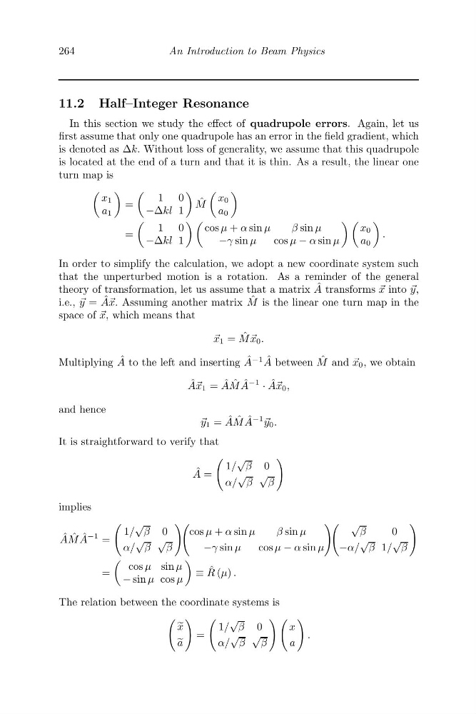
In this section we study the effect of quadrupole errors. Again, let us
first assume that only one quadrupole has an error in the field gradient, which
is denoted as Δk. Without loss of generality, we assume that this quadrupole
is located at the end of a turn and that it is thin. As a result, the linear one
turn map is
x 1
a 1
=
1 0
−Δkl 1
ˆ
M
x 0
a 0
=
1 0
−Δkl 1
cos μ + α sin μ
βsin μ
−γ sin μ
cos μ − α sin μ
x 0
a 0
.
In order to simplify the calculation, we adopt a new coordinate system such
that the unperturbed motion is a rotation. As a reminder of the general
theory of transformation, let us assume that a matrix ˆ
A transforms x into y,
i.e., y = ˆ
AA x. Assuming another matrix ˆ
M is the linear one turn map in the
space of x, which means that
x 1 = ˆ
MM x 0 .
Multiplying ˆ
A to the left and inserting ˆ
A
−1 ˆ
A between ˆ
M and x 0 , we obtain
ˆ
AA x 1 = ˆ
A ˆ
M ˆ
A
−1
· ˆ
AA x 0 ,
and hence
y 1 = ˆ
A ˆ
M ˆ
A
−1 y 0 .
It is straightforward to verify that
ˆ
A =
1/
√
β 0
α/
√
β
√
β
implies
ˆ
A ˆ
M ˆ
A
−1 =
1/
√
β 0
α/
√
β
√
β
cos μ + α sin μ
βsin μ
−γ sin μ
cos μ − α sin μ
√
β
0
−α/
√
β 1/
√
β
=
cos μ sin μ
− sin μ cos μ
≡ ˆ
R (μ) .
The relation between the coordinate systems is
x
a
=
1/
√
β 0
α/
√
β
√
β
x
a
.
An Introduction to Beam Physics
11.2 Half–Integer Resonance
In this section we study the effect of quadrupole errors. Again, let us
first assume that only one quadrupole has an error in the field gradient, which
is denoted as Δk. Without loss of generality, we assume that this quadrupole
is located at the end of a turn and that it is thin. As a result, the linear one
turn map is
x 1
a 1
=
1 0
−Δkl 1
ˆ
M
x 0
a 0
=
1 0
−Δkl 1
cos μ + α sin μ
βsin μ
−γ sin μ
cos μ − α sin μ
x 0
a 0
.
In order to simplify the calculation, we adopt a new coordinate system such
that the unperturbed motion is a rotation. As a reminder of the general
theory of transformation, let us assume that a matrix ˆ
A transforms x into y,
i.e., y = ˆ
AA x. Assuming another matrix ˆ
M is the linear one turn map in the
space of x, which means that
x 1 = ˆ
MM x 0 .
Multiplying ˆ
A to the left and inserting ˆ
A
−1 ˆ
A between ˆ
M and x 0 , we obtain
ˆ
AA x 1 = ˆ
A ˆ
M ˆ
A
−1
· ˆ
AA x 0 ,
and hence
y 1 = ˆ
A ˆ
M ˆ
A
−1 y 0 .
It is straightforward to verify that
ˆ
A =
1/
√
β 0
α/
√
β
√
β
implies
ˆ
A ˆ
M ˆ
A
−1 =
1/
√
β 0
α/
√
β
√
β
cos μ + α sin μ
βsin μ
−γ sin μ
cos μ − α sin μ
√
β
0
−α/
√
β 1/
√
β
=
cos μ sin μ
− sin μ cos μ
≡ ˆ
R (μ) .
The relation between the coordinate systems is
x
a
=
1/
√
β 0
α/
√
β
√
β
x
a
.