

Lattice Modules
221
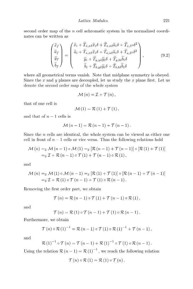
second order map of the n cell achromatic system in the normalized coordinates can be written as
⎛
⎜
⎜
⎜
⎝
x f
a f
y f
b f
⎞
⎟
⎟
⎟
⎠
=
⎛
⎜
⎜
⎜
⎜
⎝
x i +
T x,xδ
x i δ +
T x,aδ a i δ +
T x,δ 2 δ
2
a i +
T a,xδ
x i δ +
T a,aδ a i δ +
T a,δ 2 δ
2
y i +
T y,yδ
y i δ +
T y,bδ b i δ
b i +
T b,yδ
y i δ +
T b,bδ b i δ
⎞
⎟
⎟
⎟
⎟
⎠
,
(9.2)
where all geometrical terms vanish. Note that midplane symmetry is obeyed.
Since the x and y planes are decoupled, let us study the x plane first. Let us
denote the second order map of the whole system
M (n) = I + T (n) ,
that of one cell is
M (1) = R (1) + T (1) ,
and that of n − 1 cells is
M (n − 1) = R (n − 1) + T (n − 1) .
Since the n cells are identical, the whole system can be viewed as either one
cell in front of n − 1 cells or vice versa. Thus the following relations hold
M (n) = 2 M (n − 1) ◦ M (1) = 2 [R (n − 1) + T (n − 1)] ◦ [R (1) + T (1)]
= 2 I + R (n − 1) ◦ T (1) + T (n − 1) ◦ R (1) ,
and
M (n) = 2 M (1) ◦ M (n − 1) = 2 [R (1) + T (1)] ◦ [R (n − 1) + T (n − 1)]
= 2 I + R (1) ◦ T (n − 1) + T (1) ◦ R (n − 1) .
Removing the first order part, we obtain
T (n) = R (n − 1) ◦ T (1) + T (n − 1) ◦ R (1) ,
and
T (n) = R (1) ◦ T (n − 1) + T (1) ◦ R (n − 1) .
Furthermore, we obtain
T (n) ◦ R (1)
−1 = R (n − 1) ◦ T (1) ◦ R (1)
−1 + T (n − 1) ,
and
R (1)
−1 ◦ T (n) = T (n − 1) + R (1)
−1 ◦ T (1) ◦ R (n − 1) .
Using the relation R (n − 1) = R (1)
−1 , we reach the following relation
T (n) ◦ R (1) = R (1) ◦ T (n) .
221
second order map of the n cell achromatic system in the normalized coordinates can be written as
⎛
⎜
⎜
⎜
⎝
x f
a f
y f
b f
⎞
⎟
⎟
⎟
⎠
=
⎛
⎜
⎜
⎜
⎜
⎝
x i +
T x,xδ
x i δ +
T x,aδ a i δ +
T x,δ 2 δ
2
a i +
T a,xδ
x i δ +
T a,aδ a i δ +
T a,δ 2 δ
2
y i +
T y,yδ
y i δ +
T y,bδ b i δ
b i +
T b,yδ
y i δ +
T b,bδ b i δ
⎞
⎟
⎟
⎟
⎟
⎠
,
(9.2)
where all geometrical terms vanish. Note that midplane symmetry is obeyed.
Since the x and y planes are decoupled, let us study the x plane first. Let us
denote the second order map of the whole system
M (n) = I + T (n) ,
that of one cell is
M (1) = R (1) + T (1) ,
and that of n − 1 cells is
M (n − 1) = R (n − 1) + T (n − 1) .
Since the n cells are identical, the whole system can be viewed as either one
cell in front of n − 1 cells or vice versa. Thus the following relations hold
M (n) = 2 M (n − 1) ◦ M (1) = 2 [R (n − 1) + T (n − 1)] ◦ [R (1) + T (1)]
= 2 I + R (n − 1) ◦ T (1) + T (n − 1) ◦ R (1) ,
and
M (n) = 2 M (1) ◦ M (n − 1) = 2 [R (1) + T (1)] ◦ [R (n − 1) + T (n − 1)]
= 2 I + R (1) ◦ T (n − 1) + T (1) ◦ R (n − 1) .
Removing the first order part, we obtain
T (n) = R (n − 1) ◦ T (1) + T (n − 1) ◦ R (1) ,
and
T (n) = R (1) ◦ T (n − 1) + T (1) ◦ R (n − 1) .
Furthermore, we obtain
T (n) ◦ R (1)
−1 = R (n − 1) ◦ T (1) ◦ R (1)
−1 + T (n − 1) ,
and
R (1)
−1 ◦ T (n) = T (n − 1) + R (1)
−1 ◦ T (1) ◦ R (n − 1) .
Using the relation R (n − 1) = R (1)
−1 , we reach the following relation
T (n) ◦ R (1) = R (1) ◦ T (n) .