

The Linearization of the Equations of Motion
105
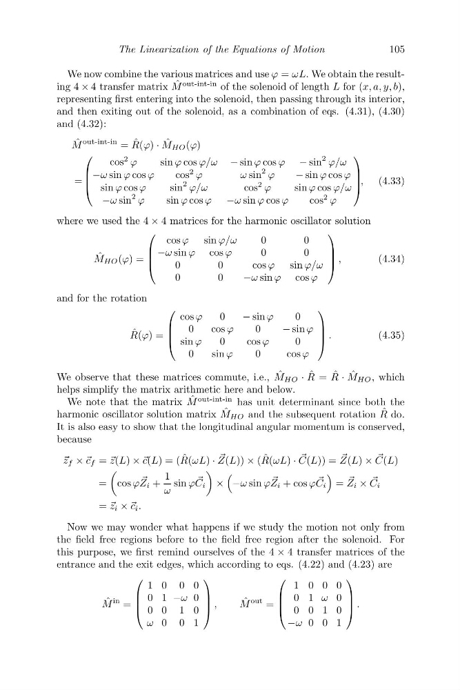
We now combine the various matrices and use ϕ = ωL. We obtain the resulting 4 × 4 transfer matrix ˆ
M
out-int-in of the solenoid of length L for (x, a, y, b),
representing first entering into the solenoid, then passing through its interior,
and then exiting out of the solenoid, as a combination of eqs. (4.31), (4.30)
and (4.32):
ˆ
M
out-int-in = ˆ
R(ϕ) · ˆ
M HO (ϕ)
=
⎛
⎜
⎜
⎝
cos
2 ϕ
sin ϕ cos ϕ/ω − sin ϕ cos ϕ − sin
2 ϕ/ω
−ω sin ϕ cos ϕ
cos
2 ϕ
ωsin
2 ϕ
− sin ϕ cos ϕ
sin ϕ cos ϕ
sin
2 ϕ/ω
cos
2 ϕ
sin ϕ cos ϕ/ω
−ω sin
2 ϕ
sin ϕ cos ϕ −ω sin ϕ cos ϕ
cos
2 ϕ
⎞
⎟
⎟
⎠ , (4.33)
where we used the 4 × 4 matrices for the harmonic oscillator solution
ˆ
M HO (ϕ) =
⎛
⎜
⎜
⎝
cos ϕ sin ϕ/ω
0
0
−ω sin ϕ cos ϕ
0
0
0
0
c o sϕ sin ϕ/ω
0
0
−ω sin ϕ cos ϕ
⎞
⎟
⎟
⎠ ,
(4.34)
and for the rotation
ˆ
R(ϕ) =
⎛
⎜
⎜
⎝
cos ϕ
0
− sin ϕ
0
0
cosϕ
0
− sin ϕ
sin ϕ
0
cosϕ
0
0
sinϕ
0
cosϕ
⎞
⎟
⎟
⎠ .
(4.35)
We observe that these matrices commute, i.e., ˆ
M HO · ˆ
R = ˆ
R · ˆ
M HO , which
helps simplify the matrix arithmetic here and below.
We note that the matrix ˆ
M
out-int-in has unit determinant since both the
harmonic oscillator solution matrix ˆ
M HO and the subsequent rotation ˆ
R do.
It is also easy to show that the longitudinal angular momentum is conserved,
because
z f × c f = z(L) × c(L) = ( ˆ
R(ωL) ·
Z(L)) × ( ˆ
R(ωL) ·
C(L)) =
Z(L) ×
C(L)
=
cos ϕ
Z i +
1
ω
sin ϕ
C i
×
−ω sin ϕ
Z i + cos ϕ
C i
=
Z i ×
C i
= z i × c i .
Now we may wonder what happens if we study the motion not only from
the field free regions before to the field free region after the solenoid. For
this purpose, we first remind ourselves of the 4 × 4 transfer matrices of the
entrance and the exit edges, which according to eqs. (4.22) and (4.23) are
ˆ
M
in =
⎛
⎜
⎜
⎝
1 0 0 0
0 1 −ω 0
0 0 1 0
ω 0 0 1
⎞
⎟
⎟
⎠ ,
ˆ
M
out =
⎛
⎜
⎜
⎝
1 0 0 0
0 1 ω 0
0 0 1 0
−ω 0 0 1
⎞
⎟
⎟
⎠ .
105
We now combine the various matrices and use ϕ = ωL. We obtain the resulting 4 × 4 transfer matrix ˆ
M
out-int-in of the solenoid of length L for (x, a, y, b),
representing first entering into the solenoid, then passing through its interior,
and then exiting out of the solenoid, as a combination of eqs. (4.31), (4.30)
and (4.32):
ˆ
M
out-int-in = ˆ
R(ϕ) · ˆ
M HO (ϕ)
=
⎛
⎜
⎜
⎝
cos
2 ϕ
sin ϕ cos ϕ/ω − sin ϕ cos ϕ − sin
2 ϕ/ω
−ω sin ϕ cos ϕ
cos
2 ϕ
ωsin
2 ϕ
− sin ϕ cos ϕ
sin ϕ cos ϕ
sin
2 ϕ/ω
cos
2 ϕ
sin ϕ cos ϕ/ω
−ω sin
2 ϕ
sin ϕ cos ϕ −ω sin ϕ cos ϕ
cos
2 ϕ
⎞
⎟
⎟
⎠ , (4.33)
where we used the 4 × 4 matrices for the harmonic oscillator solution
ˆ
M HO (ϕ) =
⎛
⎜
⎜
⎝
cos ϕ sin ϕ/ω
0
0
−ω sin ϕ cos ϕ
0
0
0
0
c o sϕ sin ϕ/ω
0
0
−ω sin ϕ cos ϕ
⎞
⎟
⎟
⎠ ,
(4.34)
and for the rotation
ˆ
R(ϕ) =
⎛
⎜
⎜
⎝
cos ϕ
0
− sin ϕ
0
0
cosϕ
0
− sin ϕ
sin ϕ
0
cosϕ
0
0
sinϕ
0
cosϕ
⎞
⎟
⎟
⎠ .
(4.35)
We observe that these matrices commute, i.e., ˆ
M HO · ˆ
R = ˆ
R · ˆ
M HO , which
helps simplify the matrix arithmetic here and below.
We note that the matrix ˆ
M
out-int-in has unit determinant since both the
harmonic oscillator solution matrix ˆ
M HO and the subsequent rotation ˆ
R do.
It is also easy to show that the longitudinal angular momentum is conserved,
because
z f × c f = z(L) × c(L) = ( ˆ
R(ωL) ·
Z(L)) × ( ˆ
R(ωL) ·
C(L)) =
Z(L) ×
C(L)
=
cos ϕ
Z i +
1
ω
sin ϕ
C i
×
−ω sin ϕ
Z i + cos ϕ
C i
=
Z i ×
C i
= z i × c i .
Now we may wonder what happens if we study the motion not only from
the field free regions before to the field free region after the solenoid. For
this purpose, we first remind ourselves of the 4 × 4 transfer matrices of the
entrance and the exit edges, which according to eqs. (4.22) and (4.23) are
ˆ
M
in =
⎛
⎜
⎜
⎝
1 0 0 0
0 1 −ω 0
0 0 1 0
ω 0 0 1
⎞
⎟
⎟
⎠ ,
ˆ
M
out =
⎛
⎜
⎜
⎝
1 0 0 0
0 1 ω 0
0 0 1 0
−ω 0 0 1
⎞
⎟
⎟
⎠ .