

h, T ∞
hθ = −k ∂y
∂θ
T( y )
∇ 2 T = 0
T 0 ⇒ θ( y )
∇
2 θ = 0
θ =T–T ∞
θ 0
⇒
Superposition
θ = θ 1 + θ 2 + θ 3
q″
∂y
q″ = −k
∂θ
hθ 1 = −k ∂y
∂θ 1
hθ 2 = −k ∂y
∂θ 2
hθ 3 = −k ∂y
∂θ 3
θ 1
= 0
∇
2 θ 1 = 0
θ 1 = 0 θ 2 = θ 2 ( y ) ∇ 2 θ = 0
2
θ 2 = 0 θ 3 = 0
∇
2 θ 3 = 0
θ 3 = θ 0
∂y
q″ = −k
∂θ 1
∂y
0 = −k
∂θ 2
∂y
0 = −k
∂θ 3
⊕
⊕
�
�
53
2-D Steady-State Heat Conduction
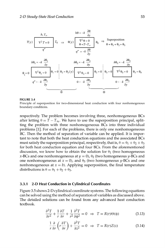
FIGURE 3.4
Principle of superposition for two-dimensional heat conduction with four nonhomogenous
boundary conditions.
respectively. The problem becomes involving three, nonhomogeneous BCs
after letting θ = T − T ∞ . We have to use the superposition principal, splitting the problem with three nonhomogeneous BCs into three individual
problems [1]. For each of the problems, there is only one nonhomogeneous
BC. Then the method of separation of variable can be applied. It is important to note that both the heat conduction equations and the associated BCs
must satisfy the superposition principal, respectively, that is, θ = θ 1 + θ 2 + θ 3
for both heat conduction equation and four BCs. From the aforementioned
discussion, we know how to obtain the solution for θ 1 (two homogeneous
x-BCs and one nonhomogeneous at y = 0), θ 2 (two homogeneous y-BCs and
one nonhomogeneous at x = 0), and θ 3 (two homogeneous y-BCs and one
nonhomogeneous at x = b). Applying superposition, the final temperature
distributions is θ = θ 1 + θ 2 + θ 3 .
3.3.1 2-D Heat Conduction in Cylindrical Coordinates
Figure 3.5 shows 2-D cylindrical coordinate systems. The following equations
can be solved using the method of separation of variables as discussed above.
The detailed solutions can be found from any advanced heat conduction
textbook.
∂ 2 T
1 ∂T
1 ∂ 2 T
+
+
= 0 ⇒ T = R(r)Θ(φ)
(3.13)
∂r 2
r ∂r
r 2 ∂φ 2
1 ∂
∂T
∂ 2 T
r
+
= 0 ⇒ T = R(r)Z(z)
(3.14)
r ∂r
∂r
∂z 2
hθ = −k ∂y
∂θ
T( y )
∇ 2 T = 0
T 0 ⇒ θ( y )
∇
2 θ = 0
θ =T–T ∞
θ 0
⇒
Superposition
θ = θ 1 + θ 2 + θ 3
q″
∂y
q″ = −k
∂θ
hθ 1 = −k ∂y
∂θ 1
hθ 2 = −k ∂y
∂θ 2
hθ 3 = −k ∂y
∂θ 3
θ 1
= 0
∇
2 θ 1 = 0
θ 1 = 0 θ 2 = θ 2 ( y ) ∇ 2 θ = 0
2
θ 2 = 0 θ 3 = 0
∇
2 θ 3 = 0
θ 3 = θ 0
∂y
q″ = −k
∂θ 1
∂y
0 = −k
∂θ 2
∂y
0 = −k
∂θ 3
⊕
⊕
�
�
53
2-D Steady-State Heat Conduction
FIGURE 3.4
Principle of superposition for two-dimensional heat conduction with four nonhomogenous
boundary conditions.
respectively. The problem becomes involving three, nonhomogeneous BCs
after letting θ = T − T ∞ . We have to use the superposition principal, splitting the problem with three nonhomogeneous BCs into three individual
problems [1]. For each of the problems, there is only one nonhomogeneous
BC. Then the method of separation of variable can be applied. It is important to note that both the heat conduction equations and the associated BCs
must satisfy the superposition principal, respectively, that is, θ = θ 1 + θ 2 + θ 3
for both heat conduction equation and four BCs. From the aforementioned
discussion, we know how to obtain the solution for θ 1 (two homogeneous
x-BCs and one nonhomogeneous at y = 0), θ 2 (two homogeneous y-BCs and
one nonhomogeneous at x = 0), and θ 3 (two homogeneous y-BCs and one
nonhomogeneous at x = b). Applying superposition, the final temperature
distributions is θ = θ 1 + θ 2 + θ 3 .
3.3.1 2-D Heat Conduction in Cylindrical Coordinates
Figure 3.5 shows 2-D cylindrical coordinate systems. The following equations
can be solved using the method of separation of variables as discussed above.
The detailed solutions can be found from any advanced heat conduction
textbook.
∂ 2 T
1 ∂T
1 ∂ 2 T
+
+
= 0 ⇒ T = R(r)Θ(φ)
(3.13)
∂r 2
r ∂r
r 2 ∂φ 2
1 ∂
∂T
∂ 2 T
r
+
= 0 ⇒ T = R(r)Z(z)
(3.14)
r ∂r
∂r
∂z 2