

0.28
f ′ =
u
1 2v
G x
2
x
0.12
0
1
4
y G x
η = x
4
1
T−T ∞
θ =
T w −T ∞
0
Pr = 0.73
1.0
10
100
1000
1
2
3
4
1
4
y G x
η = x
4
Pr = 0.73
1.0
10
100
1000
0
1
2
3
4
188
Analytical Heat Transfer
The resultant similarity momentum and energy equations are
f
"""
+ 3ff
""
− 2f
"2
+ θ = 0
(9.9)
"
θ
""
+ 3Pr f θ = 0
(9.10)
The related BCs are
f (0) = f
" (0) = 0, f
" (∞) = 0
(9.11)
θ(0) = 1, θ(∞) = 0
(9.12)
These can be solved by the fourth-order Runge–Kutta method in order
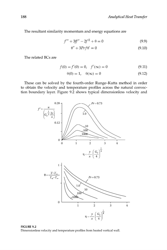
to obtain the velocity and temperature profiles across the natural convection boundary layer. Figure 9.2 shows typical dimensionless velocity and
FIGURE 9.2
Dimensionless velocity and temperature profiles from heated vertical wall.
f ′ =
u
1 2v
G x
2
x
0.12
0
1
4
y G x
η = x
4
1
T−T ∞
θ =
T w −T ∞
0
Pr = 0.73
1.0
10
100
1000
1
2
3
4
1
4
y G x
η = x
4
Pr = 0.73
1.0
10
100
1000
0
1
2
3
4
188
Analytical Heat Transfer
The resultant similarity momentum and energy equations are
f
"""
+ 3ff
""
− 2f
"2
+ θ = 0
(9.9)
"
θ
""
+ 3Pr f θ = 0
(9.10)
The related BCs are
f (0) = f
" (0) = 0, f
" (∞) = 0
(9.11)
θ(0) = 1, θ(∞) = 0
(9.12)
These can be solved by the fourth-order Runge–Kutta method in order
to obtain the velocity and temperature profiles across the natural convection boundary layer. Figure 9.2 shows typical dimensionless velocity and
FIGURE 9.2
Dimensionless velocity and temperature profiles from heated vertical wall.