

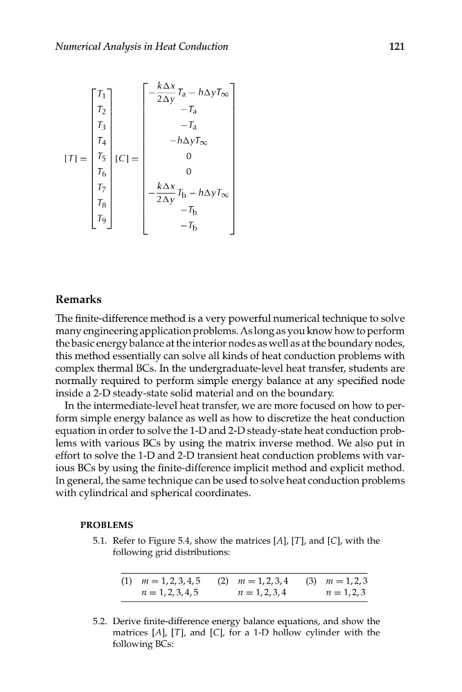
⎡
T 1
⎢
⎢ T 2
⎢
⎢
⎢T 3
⎢
⎢
⎢ T 4
⎢
⎢
[T ] = ⎢ T 5
⎢
⎢ T 6
⎢
⎢
⎢T 7
⎢
⎢
⎢ T 8
⎣
T 9
⎤
⎥
⎥
⎥
⎥
⎥
⎥
⎥
⎥
⎥
⎥
⎥
⎥
⎥
⎥
⎥
⎥
⎥
⎥
⎥
⎦
[C ] =
⎡ k Δx
−
T a − hΔyT ∞
⎢ 2Δy
⎢
⎢
−T a
⎢
⎢
⎢
−T a
⎢
⎢
⎢
−hΔyT ∞
⎢
⎢
0
⎢
⎢
⎢
0
⎢
⎢
⎢ k Δx
⎢−
T b − hΔyT ∞
⎢ 2Δy
⎢
⎢
−T b
⎣
−T b
⎤
⎥
⎥
⎥
⎥
⎥
⎥
⎥
⎥
⎥
⎥
⎥
⎥
⎥
⎥
⎥
⎥
⎥
⎥
⎥
⎥
⎥
⎦
121
Numerical Analysis in Heat Conduction
Remarks
The finite-difference method is a very powerful numerical technique to solve
many engineering application problems. As long as you know how to perform
the basic energy balance at the interior nodes as well as at the boundary nodes,
this method essentially can solve all kinds of heat conduction problems with
complex thermal BCs. In the undergraduate-level heat transfer, students are
normally required to perform simple energy balance at any specified node
inside a 2-D steady-state solid material and on the boundary.
In the intermediate-level heat transfer, we are more focused on how to perform simple energy balance as well as how to discretize the heat conduction
equation in order to solve the 1-D and 2-D steady-state heat conduction problems with various BCs by using the matrix inverse method. We also put in
effort to solve the 1-D and 2-D transient heat conduction problems with various BCs by using the finite-difference implicit method and explicit method.
In general, the same technique can be used to solve heat conduction problems
with cylindrical and spherical coordinates.
PROBLEMS
5.1. Refer to Figure 5.4, show the matrices [A], [T], and [C], with the
following grid distributions:
(1) m = 1, 2, 3, 4, 5
(2) m = 1, 2, 3, 4
(3) m = 1, 2, 3
n = 1, 2, 3, 4, 5
n = 1, 2, 3, 4
n = 1, 2, 3
5.2. Derive finite-difference energy balance equations, and show the
matrices [A], [T], and [C], for a 1-D hollow cylinder with the
following BCs:
T 1
⎢
⎢ T 2
⎢
⎢
⎢T 3
⎢
⎢
⎢ T 4
⎢
⎢
[T ] = ⎢ T 5
⎢
⎢ T 6
⎢
⎢
⎢T 7
⎢
⎢
⎢ T 8
⎣
T 9
⎤
⎥
⎥
⎥
⎥
⎥
⎥
⎥
⎥
⎥
⎥
⎥
⎥
⎥
⎥
⎥
⎥
⎥
⎥
⎥
⎦
[C ] =
⎡ k Δx
−
T a − hΔyT ∞
⎢ 2Δy
⎢
⎢
−T a
⎢
⎢
⎢
−T a
⎢
⎢
⎢
−hΔyT ∞
⎢
⎢
0
⎢
⎢
⎢
0
⎢
⎢
⎢ k Δx
⎢−
T b − hΔyT ∞
⎢ 2Δy
⎢
⎢
−T b
⎣
−T b
⎤
⎥
⎥
⎥
⎥
⎥
⎥
⎥
⎥
⎥
⎥
⎥
⎥
⎥
⎥
⎥
⎥
⎥
⎥
⎥
⎥
⎥
⎦
121
Numerical Analysis in Heat Conduction
Remarks
The finite-difference method is a very powerful numerical technique to solve
many engineering application problems. As long as you know how to perform
the basic energy balance at the interior nodes as well as at the boundary nodes,
this method essentially can solve all kinds of heat conduction problems with
complex thermal BCs. In the undergraduate-level heat transfer, students are
normally required to perform simple energy balance at any specified node
inside a 2-D steady-state solid material and on the boundary.
In the intermediate-level heat transfer, we are more focused on how to perform simple energy balance as well as how to discretize the heat conduction
equation in order to solve the 1-D and 2-D steady-state heat conduction problems with various BCs by using the matrix inverse method. We also put in
effort to solve the 1-D and 2-D transient heat conduction problems with various BCs by using the finite-difference implicit method and explicit method.
In general, the same technique can be used to solve heat conduction problems
with cylindrical and spherical coordinates.
PROBLEMS
5.1. Refer to Figure 5.4, show the matrices [A], [T], and [C], with the
following grid distributions:
(1) m = 1, 2, 3, 4, 5
(2) m = 1, 2, 3, 4
(3) m = 1, 2, 3
n = 1, 2, 3, 4, 5
n = 1, 2, 3, 4
n = 1, 2, 3
5.2. Derive finite-difference energy balance equations, and show the
matrices [A], [T], and [C], for a 1-D hollow cylinder with the
following BCs: