

111
Numerical Analysis in Heat Conduction
Example 5.2
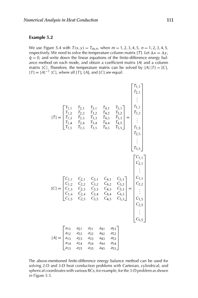
We use Figure 5.4 with T (x, y ) = T m,n , when m = 1, 2, 3, 4, 5, n = 1, 2, 3, 4, 5,
respectively. We need to solve the temperature column matrix [T ]. Let Δx = Δy ,
q ˙ = 0, and write down the linear equations of the finite-difference energy balance method on each mode, and obtain a coefficient matrix [A] and a column
matrix [C ]. Therefore, the temperature matrix can be solved by [A] [T ] = [C ],
[T ] = [A] −1 [C ], where all [T ], [A], and [C ] are equal:
T 1,1
⎡
T 2,1 T 3,1 T 4,1 T 5,1
⎤
⎢
⎢ T 1,2 T 2,2 T 3,2 T 4,2 T 5,2 ⎥
⎥
[T ] = ⎢
⎢ T 1,3 T 2,3 T 3,3 T 4,3 T 5,3 ⎥
⎥ =
⎣ T 1,4 T 2,4 T 3,4 T 4,4 T 4,5 ⎦
T 1,5 T 2,5 T 3,5 T 4,5 T 5,5
⎡
C 1,1 C 2,1 C 3,1 C 4,1 C 5,1
⎤
⎢
⎢ C 1,2 C 2,2 C 3,2 C 4,2 C 5,2 ⎥
⎥
[C ] = ⎢
⎢ C 1,3 C 2,3 C 3,3 C 4,3 C 5,3 ⎥
⎥ =
⎣ C 1,4 C 2,4 C 3,4 C 4,4 C 4,5 ⎦
C 1,5 C 2,5 C 3,5 C 4,5 C 5,5
⎡
⎤
a 11 a 21 a 31 a 41 a 51
⎢ a 12 a 22 a 32 a 42 a 52 ⎥
⎢
⎥
[A] = ⎢ a 13 a 23 a 33 a 43 a 53 ⎥
⎢
⎥
⎣ a 14 a 24 a 34 a 44 a 54 ⎦
a 15 a 25 a 35 a 45 a 55
⎡
T 1,1
⎢
⎢ T 2,1
⎢
⎢ .
⎢ . .
⎢
⎢
⎢ T 1,1
⎢
⎢ T 2,2
⎢
⎢ .
⎢ .
⎢ .
⎢
⎢
⎢ T 1,5
⎢
⎢ T 2,5
⎢
⎢ .
⎢ . .
T 5,5
⎣
⎤
⎥
⎥
⎥
⎥
⎥
⎥
⎥
⎥
⎥
⎥
⎥
⎥
⎥
⎥
⎥
⎥
⎥
⎥
⎥
⎥
⎥
⎥
⎦
⎡
C 1,1
⎢
⎢ C 2,1
⎢
⎢ .
⎢ . .
⎢
⎢
⎢ C 1,1
⎢
⎢ C 2,2
⎢
⎢ .
⎢ .
⎢ .
⎢
⎢
⎢ C 1,5
⎢
⎢ C 2,5
⎢
⎢ .
⎢ . .
C 5,5
⎣
⎤
⎥
⎥
⎥
⎥
⎥
⎥
⎥
⎥
⎥
⎥
⎥
⎥
⎥
⎥
⎥
⎥
⎥
⎥
⎥
⎥
⎥
⎥
⎦
The above-mentioned finite-difference energy balance method can be used for
solving 2-D and 3-D heat conduction problems with Cartesian, cylindrical, and
spherical coordinates with various BCs; for example, for the 3-D problem as shown
in Figure 5.5.
Numerical Analysis in Heat Conduction
Example 5.2
We use Figure 5.4 with T (x, y ) = T m,n , when m = 1, 2, 3, 4, 5, n = 1, 2, 3, 4, 5,
respectively. We need to solve the temperature column matrix [T ]. Let Δx = Δy ,
q ˙ = 0, and write down the linear equations of the finite-difference energy balance method on each mode, and obtain a coefficient matrix [A] and a column
matrix [C ]. Therefore, the temperature matrix can be solved by [A] [T ] = [C ],
[T ] = [A] −1 [C ], where all [T ], [A], and [C ] are equal:
T 1,1
⎡
T 2,1 T 3,1 T 4,1 T 5,1
⎤
⎢
⎢ T 1,2 T 2,2 T 3,2 T 4,2 T 5,2 ⎥
⎥
[T ] = ⎢
⎢ T 1,3 T 2,3 T 3,3 T 4,3 T 5,3 ⎥
⎥ =
⎣ T 1,4 T 2,4 T 3,4 T 4,4 T 4,5 ⎦
T 1,5 T 2,5 T 3,5 T 4,5 T 5,5
⎡
C 1,1 C 2,1 C 3,1 C 4,1 C 5,1
⎤
⎢
⎢ C 1,2 C 2,2 C 3,2 C 4,2 C 5,2 ⎥
⎥
[C ] = ⎢
⎢ C 1,3 C 2,3 C 3,3 C 4,3 C 5,3 ⎥
⎥ =
⎣ C 1,4 C 2,4 C 3,4 C 4,4 C 4,5 ⎦
C 1,5 C 2,5 C 3,5 C 4,5 C 5,5
⎡
⎤
a 11 a 21 a 31 a 41 a 51
⎢ a 12 a 22 a 32 a 42 a 52 ⎥
⎢
⎥
[A] = ⎢ a 13 a 23 a 33 a 43 a 53 ⎥
⎢
⎥
⎣ a 14 a 24 a 34 a 44 a 54 ⎦
a 15 a 25 a 35 a 45 a 55
⎡
T 1,1
⎢
⎢ T 2,1
⎢
⎢ .
⎢ . .
⎢
⎢
⎢ T 1,1
⎢
⎢ T 2,2
⎢
⎢ .
⎢ .
⎢ .
⎢
⎢
⎢ T 1,5
⎢
⎢ T 2,5
⎢
⎢ .
⎢ . .
T 5,5
⎣
⎤
⎥
⎥
⎥
⎥
⎥
⎥
⎥
⎥
⎥
⎥
⎥
⎥
⎥
⎥
⎥
⎥
⎥
⎥
⎥
⎥
⎥
⎥
⎦
⎡
C 1,1
⎢
⎢ C 2,1
⎢
⎢ .
⎢ . .
⎢
⎢
⎢ C 1,1
⎢
⎢ C 2,2
⎢
⎢ .
⎢ .
⎢ .
⎢
⎢
⎢ C 1,5
⎢
⎢ C 2,5
⎢
⎢ .
⎢ . .
C 5,5
⎣
⎤
⎥
⎥
⎥
⎥
⎥
⎥
⎥
⎥
⎥
⎥
⎥
⎥
⎥
⎥
⎥
⎥
⎥
⎥
⎥
⎥
⎥
⎥
⎦
The above-mentioned finite-difference energy balance method can be used for
solving 2-D and 3-D heat conduction problems with Cartesian, cylindrical, and
spherical coordinates with various BCs; for example, for the 3-D problem as shown
in Figure 5.5.