

[T ] = [A] −1 [C ]
[A] =
⎡
⎢
⎢
⎢
⎢
⎢
⎢
⎢
⎢
⎢
⎢
⎢
⎢
⎢
⎢
⎣
−4
1
1
0
0
0
2
−4
0
1
0
0
1
0
−4
1
1
0
0
1
2
−4
0
1
0
0
1
0
−4
1
0
0
0
1
2
−4
0
0
0
0
2
0
0
0
0
0
0
1
[C ] =
⎡
⎢
⎢
⎢
⎢
⎢
⎢
⎢
⎢
⎢
⎢
⎢
⎢
⎢
⎣
−T s
−T s
−T s
0
−T s
0
−T s −
2h
k
ΔxT ∞
−
h
k
ΔxT ∞
⎤
⎥
⎥
⎥
⎥
⎥
⎥
⎥
⎥
⎥
⎥
⎥
⎥
⎥
⎦
[T ] =
⎡
⎢
⎢
⎢
⎢
⎢
⎢
⎢
⎢
⎢
⎢
⎣
T 1
T 2
T 3
T 4
T 5
T 6
T 7
T 8
⎤
⎥
⎥
⎥
⎥
⎥
⎥
⎥
⎥
⎥
⎥
⎦
0
0
0
0
1
0
−
�
4 +
2h
k
Δx
�
1
0
0
0
0
0
1
1
−
�
2 +
h
k
Δx
�
⎤
⎥
⎥
⎥
⎥
⎥
⎥
⎥
⎥
⎥
⎥
⎥
⎥
⎥
⎥
⎦
110
Analytical Heat Transfer
T s
5
1
1
2
3
3
4
6
8
7
7
T s
T s
5
T ∞ , h
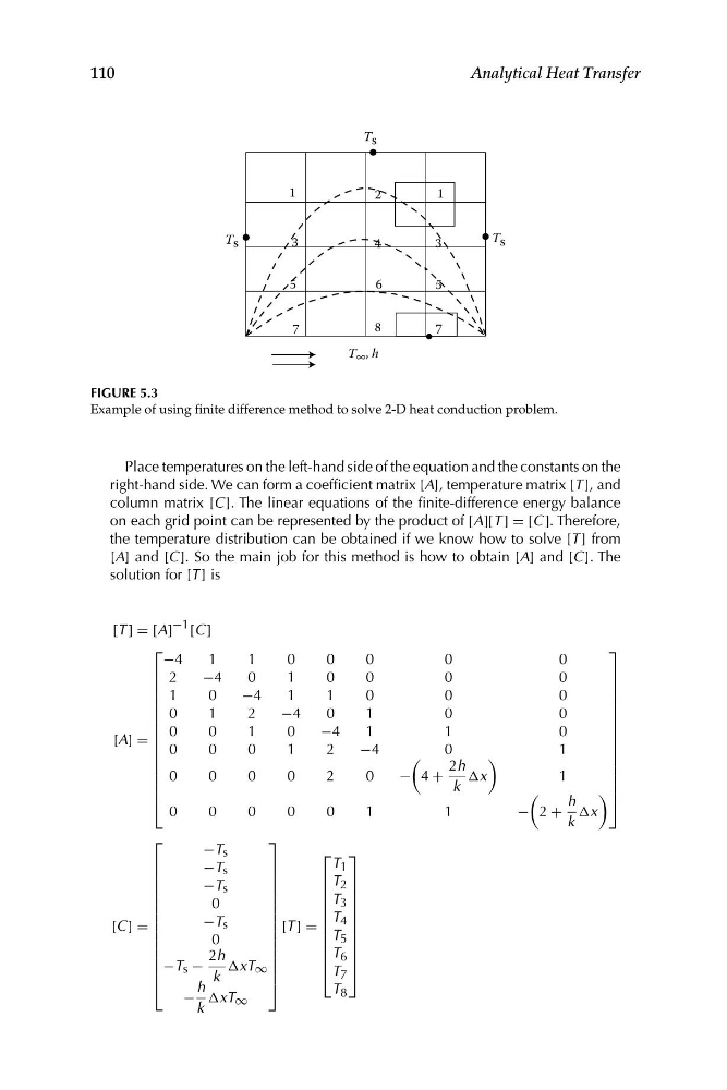
FIGURE 5.3
Example of using finite difference method to solve 2-D heat conduction problem.
Place temperatures on the left-hand side of the equation and the constants on the
right-hand side. We can form a coefficient matrix [A], temperature matrix [T ], and
column matrix [C ]. The linear equations of the finite-difference energy balance
on each grid point can be represented by the product of [A][T ] = [C ]. Therefore,
the temperature distribution can be obtained if we know how to solve [T ] from
[A] and [C ]. So the main job for this method is how to obtain [A] and [C ]. The
solution for [T ] is
[A] =
⎡
⎢
⎢
⎢
⎢
⎢
⎢
⎢
⎢
⎢
⎢
⎢
⎢
⎢
⎢
⎣
−4
1
1
0
0
0
2
−4
0
1
0
0
1
0
−4
1
1
0
0
1
2
−4
0
1
0
0
1
0
−4
1
0
0
0
1
2
−4
0
0
0
0
2
0
0
0
0
0
0
1
[C ] =
⎡
⎢
⎢
⎢
⎢
⎢
⎢
⎢
⎢
⎢
⎢
⎢
⎢
⎢
⎣
−T s
−T s
−T s
0
−T s
0
−T s −
2h
k
ΔxT ∞
−
h
k
ΔxT ∞
⎤
⎥
⎥
⎥
⎥
⎥
⎥
⎥
⎥
⎥
⎥
⎥
⎥
⎥
⎦
[T ] =
⎡
⎢
⎢
⎢
⎢
⎢
⎢
⎢
⎢
⎢
⎢
⎣
T 1
T 2
T 3
T 4
T 5
T 6
T 7
T 8
⎤
⎥
⎥
⎥
⎥
⎥
⎥
⎥
⎥
⎥
⎥
⎦
0
0
0
0
1
0
−
�
4 +
2h
k
Δx
�
1
0
0
0
0
0
1
1
−
�
2 +
h
k
Δx
�
⎤
⎥
⎥
⎥
⎥
⎥
⎥
⎥
⎥
⎥
⎥
⎥
⎥
⎥
⎥
⎦
110
Analytical Heat Transfer
T s
5
1
1
2
3
3
4
6
8
7
7
T s
T s
5
T ∞ , h
FIGURE 5.3
Example of using finite difference method to solve 2-D heat conduction problem.
Place temperatures on the left-hand side of the equation and the constants on the
right-hand side. We can form a coefficient matrix [A], temperature matrix [T ], and
column matrix [C ]. The linear equations of the finite-difference energy balance
on each grid point can be represented by the product of [A][T ] = [C ]. Therefore,
the temperature distribution can be obtained if we know how to solve [T ] from
[A] and [C ]. So the main job for this method is how to obtain [A] and [C ]. The
solution for [T ] is