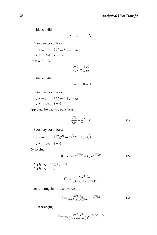
Initial condition:

t = 0; T = T i .

Boundary conditions:
i. x = 0; −k ∂θ = h(θ ∞ − θ 0 )
∂x
ii. x → ∞; T = T i
Let θ = T − T i ,
∂ 2 θ
1 ∂θ
=
∂x 2
α ∂t
Initial condition:

t = 0; θ = 0

Boundary conditions:
i. x = 0; −k ∂θ = h(θ ∞ − θ 0 )
∂x
ii. x → ∞; θ = 0
Applying the Laplace transform,
∂ 2 θ ˜
s
− θ ˜ = 0
(1)
∂x 2
α
Boundary conditions:
(
)
−k
dθ ˜ (0,t )
θ ∞
i. x = 0;
dx
= h s − θ ˜ (0, t )
˜
ii. x → ∞; θ = 0
By solving,
√
√
−
s/αx
θ ˜ = C 1 e s/αx + C 2 e
(2)
Applying BC (ii), C 2 = 0.

Applying BC (i),

(h/k )θ ∞
C 1 =
√
((h/k ) + ( s/α))s
Substituting this into above (2),
˜
(h/k )θ ∞
−
√
s/αx
θ =
√
e
(3)
((h/k )+( s/α))s
By rearranging,
√
√ √
˜
(h/k ) α
−(x/ α) s
θ = θ ∞ (
√ √ ) e
(h/k ) α+ s s
98
Analytical Heat Transfer