

3.0
1.6
1.4
2.5
E
0 (×10
−6
)
E
0 (×10 −4
)
1.2
1.0
0.8
0.6
2.0
1.5
1.0
0.4
0.5
0.2
0
10
2
10 3
10 4
10 5
10 6
10 7
0
10 0
10 1
10 2
10 3
10 4
10 5
ω = 2πf
ω = 2πf
(a)
(b)
46
Electromagnetic Fields in Biological Systems
Normalized amplitude
0.2
0.4
0.6
0.8
1.0
−3t 1 −2t 1
−t 1
0
t 1
2t 1
3t 1
Time
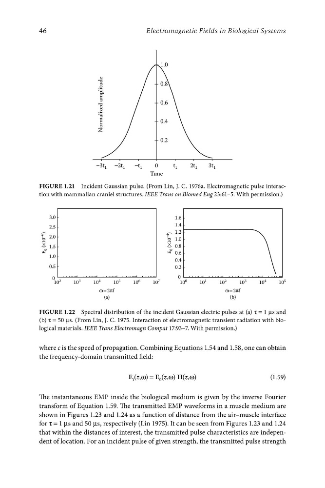
FigurE 1.21 Incident Gaussian pulse. (From Lin, J. C. 1976a. Electromagnetic pulse interaction with mammalian craniel structures. IEEE Trans on Biomed Eng 23:61–5. With permission.)
FigurE 1.22 Spectral distribution of the incident Gaussian electric pulses at (a) τ = 1 μs and
(b) τ = 50 μs. (From Lin, J. C. 1975. Interaction of electromagnetic transient radiation with biological materials. IEEE Trans Electromagn Compat 17:93–7. With permission.)
where c is the speed of propagation. Combining Equations 1.54 and 1.58, one can obtain
the frequency-domain transmitted field:
E t (z,ω) = E 0 (z,ω) H(z,ω)
(1.59)
The instantaneous EMP inside the biological medium is given by the inverse Fourier
transform of Equation 1.59. The transmitted EMP waveforms in a muscle medium are
shown in Figures 1.23 and 1.24 as a function of distance from the air–muscle interface
for τ = 1 μs and 50 μs, respectively (Lin 1975). It can be seen from Figures 1.23 and 1.24
that within the distances of interest, the transmitted pulse characteristics are independent of location. For an incident pulse of given strength, the transmitted pulse strength
1.6
1.4
2.5
E
0 (×10
−6
)
E
0 (×10 −4
)
1.2
1.0
0.8
0.6
2.0
1.5
1.0
0.4
0.5
0.2
0
10
2
10 3
10 4
10 5
10 6
10 7
0
10 0
10 1
10 2
10 3
10 4
10 5
ω = 2πf
ω = 2πf
(a)
(b)
46
Electromagnetic Fields in Biological Systems
Normalized amplitude
0.2
0.4
0.6
0.8
1.0
−3t 1 −2t 1
−t 1
0
t 1
2t 1
3t 1
Time
FigurE 1.21 Incident Gaussian pulse. (From Lin, J. C. 1976a. Electromagnetic pulse interaction with mammalian craniel structures. IEEE Trans on Biomed Eng 23:61–5. With permission.)
FigurE 1.22 Spectral distribution of the incident Gaussian electric pulses at (a) τ = 1 μs and
(b) τ = 50 μs. (From Lin, J. C. 1975. Interaction of electromagnetic transient radiation with biological materials. IEEE Trans Electromagn Compat 17:93–7. With permission.)
where c is the speed of propagation. Combining Equations 1.54 and 1.58, one can obtain
the frequency-domain transmitted field:
E t (z,ω) = E 0 (z,ω) H(z,ω)
(1.59)
The instantaneous EMP inside the biological medium is given by the inverse Fourier
transform of Equation 1.59. The transmitted EMP waveforms in a muscle medium are
shown in Figures 1.23 and 1.24 as a function of distance from the air–muscle interface
for τ = 1 μs and 50 μs, respectively (Lin 1975). It can be seen from Figures 1.23 and 1.24
that within the distances of interest, the transmitted pulse characteristics are independent of location. For an incident pulse of given strength, the transmitted pulse strength