

I s (r = r s , θ = 0, z = 0)
r
ε o , σ o
ε i , σ i
ε m , σ m
5 μm
5 nm
Z
92
Electromagnetic Fields in Biological Systems
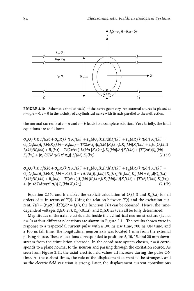
Figure 2.10 Schematic (not to scale) of the nerve geometry. An external source is placed at
r = r s , θ = 0, z = 0 in the vicinity of a cylindrical nerve with its axis parallel to the z-direction.
the normal currents at r = a and r = b leads to a complete solution. Very briefly, the final
equations are as follows:
σ m Q 0 (k,t) I 0 ‘(kb) + σ m R 0 (k,t) K 0 ‘(kb) + ε m {dQ 0 (k,t)/dt}I 0 ‘(kb) + ε m {dR 0 (k,t)/dt} K 0 ‘(kb) =
σ 0 [Q 0 (k,t)I 0 (kb)/K 0 (kb) + R
2
0 (k,t) − T/(2π σ o )]I 0 (kb) [K 0 (k r s )/K 0 (kb)]K 0 ‘(kb) + ε o {d[Q 0 (k,t)
I 0 (kb)/K 0 (kb) + R 0 (k,t) − T/(2π 2 σ o )]I
2
0 (kb) [K 0 (k r s )/K 0 (kb)]/dt}K 0 ‘(kb) + {T/(2π )}I 0 ‘(kb)
K 0 (kr s ) + {ε o (dT/dt)/(2π 2 σ 0 )} I 0 ‘(kb) K 0 (kr s )
(2.15a)
σ m Q n (k,t) I n ‘(kb) + σ m R n (k,t) K n ‘(kb) + ε m {dQ n (k,t)/dt}I n ‘(kb) + ε m {dR n (k,t)/dt} K n ‘(kb) =
σ 0 [Q n (k,t)I n (kb)/K n (kb) + R (k,t) − T/(π 2
n
σ o )]I n (kb) [K n (k r s )/K n (kb)]K n ‘(kb) + ε o {d[Q n (k,t)
I n (kb)/K n (kb) + R n (k,t) − T/(π 2 σ o )]I n (kb) [K n (k r s )/K n (kb)]/dt}K b) + {T/π 2
n ‘(k
}I n ‘(kb) K n (kr s )
+ {ε o (dT/dt)/(π 2 σ 0 )} I n ‘(kb) K n (kr s )
(2.15b)
Equation 2.15a and b enables the explicit calculation of Q n (k,t) and R n (k,t) for all
orders of n, in terms of T(t). Using the relation between T(t) and the excitation current, T(t) + (ε o /σ o ) dT(t)/dt = I s (t), the function T(t) can be obtained. Hence, the timedependent voltages φ i (r,θ,z,t), φ m (r,θ,z,t), and φ o (r,θ,z,t) can all be fully determined.
Magnitudes of the axial electric field inside the cylindrical neuron structure (i.e., at
r = 0) at four different z-locations are shown in Figure 2.11. The results shown were in
response to a trapezoidal current pulse with a 100 ns rise time, 700 ns ON time, and
a 100 ns fall time. The longitudinal neuron axis was located 1 mm from the external
pulsing source. These z-locations corresponded to positions 5, 10, 15, and 20 mm downstream from the stimulation electrode. In the coordinate system chosen, z = 0 corresponds to a plane normal to the neuron and passing through the excitation source. As
seen from Figure 2.11, the axial electric field values all increase during the pulse ON
time. At the earliest times, the role of the displacement current is the strongest, and
so the electric field variation is strong. Later, the displacement current contributions
r
ε o , σ o
ε i , σ i
ε m , σ m
5 μm
5 nm
Z
92
Electromagnetic Fields in Biological Systems
Figure 2.10 Schematic (not to scale) of the nerve geometry. An external source is placed at
r = r s , θ = 0, z = 0 in the vicinity of a cylindrical nerve with its axis parallel to the z-direction.
the normal currents at r = a and r = b leads to a complete solution. Very briefly, the final
equations are as follows:
σ m Q 0 (k,t) I 0 ‘(kb) + σ m R 0 (k,t) K 0 ‘(kb) + ε m {dQ 0 (k,t)/dt}I 0 ‘(kb) + ε m {dR 0 (k,t)/dt} K 0 ‘(kb) =
σ 0 [Q 0 (k,t)I 0 (kb)/K 0 (kb) + R
2
0 (k,t) − T/(2π σ o )]I 0 (kb) [K 0 (k r s )/K 0 (kb)]K 0 ‘(kb) + ε o {d[Q 0 (k,t)
I 0 (kb)/K 0 (kb) + R 0 (k,t) − T/(2π 2 σ o )]I
2
0 (kb) [K 0 (k r s )/K 0 (kb)]/dt}K 0 ‘(kb) + {T/(2π )}I 0 ‘(kb)
K 0 (kr s ) + {ε o (dT/dt)/(2π 2 σ 0 )} I 0 ‘(kb) K 0 (kr s )
(2.15a)
σ m Q n (k,t) I n ‘(kb) + σ m R n (k,t) K n ‘(kb) + ε m {dQ n (k,t)/dt}I n ‘(kb) + ε m {dR n (k,t)/dt} K n ‘(kb) =
σ 0 [Q n (k,t)I n (kb)/K n (kb) + R (k,t) − T/(π 2
n
σ o )]I n (kb) [K n (k r s )/K n (kb)]K n ‘(kb) + ε o {d[Q n (k,t)
I n (kb)/K n (kb) + R n (k,t) − T/(π 2 σ o )]I n (kb) [K n (k r s )/K n (kb)]/dt}K b) + {T/π 2
n ‘(k
}I n ‘(kb) K n (kr s )
+ {ε o (dT/dt)/(π 2 σ 0 )} I n ‘(kb) K n (kr s )
(2.15b)
Equation 2.15a and b enables the explicit calculation of Q n (k,t) and R n (k,t) for all
orders of n, in terms of T(t). Using the relation between T(t) and the excitation current, T(t) + (ε o /σ o ) dT(t)/dt = I s (t), the function T(t) can be obtained. Hence, the timedependent voltages φ i (r,θ,z,t), φ m (r,θ,z,t), and φ o (r,θ,z,t) can all be fully determined.
Magnitudes of the axial electric field inside the cylindrical neuron structure (i.e., at
r = 0) at four different z-locations are shown in Figure 2.11. The results shown were in
response to a trapezoidal current pulse with a 100 ns rise time, 700 ns ON time, and
a 100 ns fall time. The longitudinal neuron axis was located 1 mm from the external
pulsing source. These z-locations corresponded to positions 5, 10, 15, and 20 mm downstream from the stimulation electrode. In the coordinate system chosen, z = 0 corresponds to a plane normal to the neuron and passing through the excitation source. As
seen from Figure 2.11, the axial electric field values all increase during the pulse ON
time. At the earliest times, the role of the displacement current is the strongest, and
so the electric field variation is strong. Later, the displacement current contributions