

91
Pulsed Electric Fields in Biological Cells and Membranes
(a)
(b)
(c)
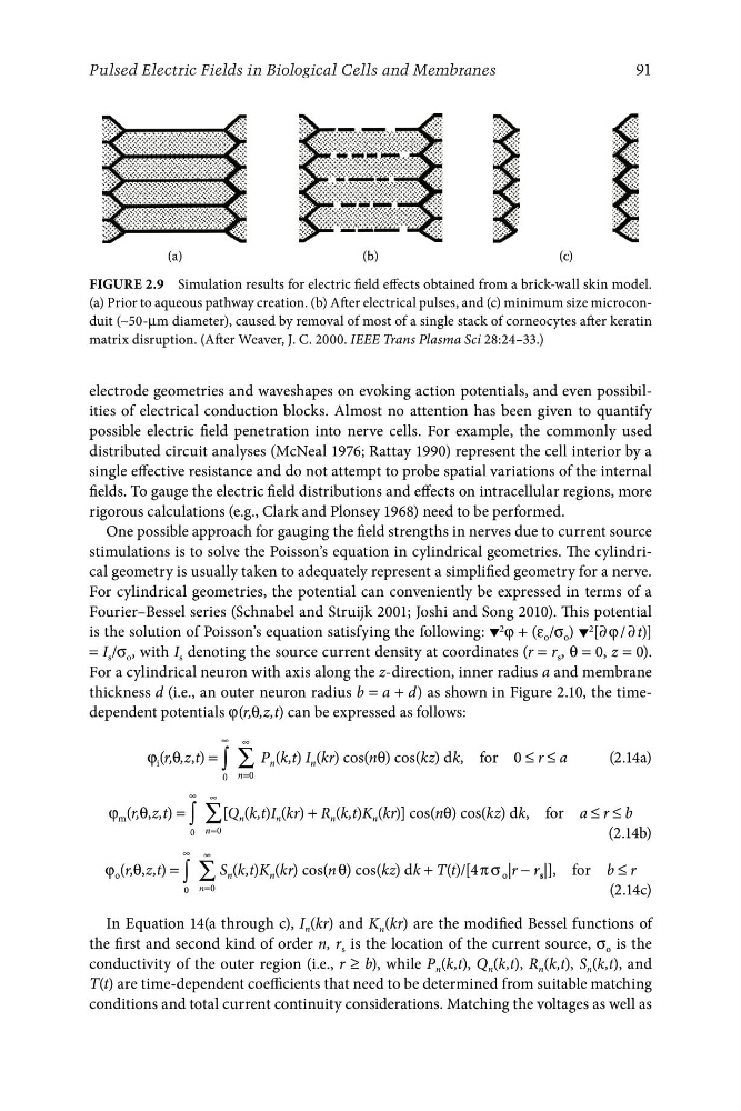
Figure 2.9 Simulation results for electric field effects obtained from a brick-wall skin model.
(a) Prior to aqueous pathway creation. (b) After electrical pulses, and (c) minimum size microconduit (∼50-μm diameter), caused by removal of most of a single stack of corneocytes after keratin
matrix disruption. (After Weaver, J. C. 2000. IEEE Trans Plasma Sci 28:24–33.)
electrode geometries and waveshapes on evoking action potentials, and even possibilities of electrical conduction blocks. Almost no attention has been given to quantify
possible electric field penetration into nerve cells. For example, the commonly used
distributed circuit analyses (McNeal 1976; Rattay 1990) represent the cell interior by a
single effective resistance and do not attempt to probe spatial variations of the internal
fields. To gauge the electric field distributions and effects on intracellular regions, more
rigorous calculations (e.g., Clark and Plonsey 1968) need to be performed.
One possible approach for gauging the field strengths in nerves due to current source
stimulations is to solve the Poisson’s equation in cylindrical geometries. The cylindrical geometry is usually taken to adequately represent a simplified geometry for a nerve.
For cylindrical geometries, the potential can conveniently be expressed in terms of a
Fourier–Bessel series (Schnabel and Struijk 2001; Joshi and Song 2010). This potential
is the solution of Poisson’s equation satisfying the following: ▾ 2 φ + (ε o /σ o ) ▾ 2 [∂ φ / ∂ t)]
= I s /σ o , with I s denoting the source current density at coordinates (r = r s , θ = 0, z = 0).
For a cylindrical neuron with axis along the z-direction, inner radius a and membrane
thickness d (i.e., an outer neuron radius b = a + d) as shown in Figure 2.10, the timedependent potentials φ(r,θ,z,t) can be expressed as follows:
∞
φ
∫ ∑
∞
i (r,θ,z,t) =
P n (k,t) I n (kr) cos(nθ) cos(kz) dk, for 0 ≤ r ≤ a
(2.14a)
0 n=0
∞ ∞
φ m (r,θ,z,t) = ∫ ∑ [Q n (k,t)I n (kr) + R n (k,t)K n (kr)] cos(nθ) cos(kz) dk, for a ≤ r ≤ b
0 n=0
(2.14b)
∞ ∞
φ o (r,θ,z,t) = ∫ ∑ S n (k,t)K n (kr) cos(n θ) cos(kz) dk + T(t)/[4 π σ o |r − r s |], for b ≤ r
0 n=0
(2.14c)
In Equation 14(a through c), I n (kr) and K n (kr) are the modified Bessel functions of
the first and second kind of order n, r s is the location of the current source, σ o is the
conductivity of the outer region (i.e., r ≥ b), while P n (k,t), Q n (k,t), R n (k,t), S n (k,t), and
T(t) are time-dependent coefficients that need to be determined from suitable matching
conditions and total current continuity considerations. Matching the voltages as well as
Pulsed Electric Fields in Biological Cells and Membranes
(a)
(b)
(c)
Figure 2.9 Simulation results for electric field effects obtained from a brick-wall skin model.
(a) Prior to aqueous pathway creation. (b) After electrical pulses, and (c) minimum size microconduit (∼50-μm diameter), caused by removal of most of a single stack of corneocytes after keratin
matrix disruption. (After Weaver, J. C. 2000. IEEE Trans Plasma Sci 28:24–33.)
electrode geometries and waveshapes on evoking action potentials, and even possibilities of electrical conduction blocks. Almost no attention has been given to quantify
possible electric field penetration into nerve cells. For example, the commonly used
distributed circuit analyses (McNeal 1976; Rattay 1990) represent the cell interior by a
single effective resistance and do not attempt to probe spatial variations of the internal
fields. To gauge the electric field distributions and effects on intracellular regions, more
rigorous calculations (e.g., Clark and Plonsey 1968) need to be performed.
One possible approach for gauging the field strengths in nerves due to current source
stimulations is to solve the Poisson’s equation in cylindrical geometries. The cylindrical geometry is usually taken to adequately represent a simplified geometry for a nerve.
For cylindrical geometries, the potential can conveniently be expressed in terms of a
Fourier–Bessel series (Schnabel and Struijk 2001; Joshi and Song 2010). This potential
is the solution of Poisson’s equation satisfying the following: ▾ 2 φ + (ε o /σ o ) ▾ 2 [∂ φ / ∂ t)]
= I s /σ o , with I s denoting the source current density at coordinates (r = r s , θ = 0, z = 0).
For a cylindrical neuron with axis along the z-direction, inner radius a and membrane
thickness d (i.e., an outer neuron radius b = a + d) as shown in Figure 2.10, the timedependent potentials φ(r,θ,z,t) can be expressed as follows:
∞
φ
∫ ∑
∞
i (r,θ,z,t) =
P n (k,t) I n (kr) cos(nθ) cos(kz) dk, for 0 ≤ r ≤ a
(2.14a)
0 n=0
∞ ∞
φ m (r,θ,z,t) = ∫ ∑ [Q n (k,t)I n (kr) + R n (k,t)K n (kr)] cos(nθ) cos(kz) dk, for a ≤ r ≤ b
0 n=0
(2.14b)
∞ ∞
φ o (r,θ,z,t) = ∫ ∑ S n (k,t)K n (kr) cos(n θ) cos(kz) dk + T(t)/[4 π σ o |r − r s |], for b ≤ r
0 n=0
(2.14c)
In Equation 14(a through c), I n (kr) and K n (kr) are the modified Bessel functions of
the first and second kind of order n, r s is the location of the current source, σ o is the
conductivity of the outer region (i.e., r ≥ b), while P n (k,t), Q n (k,t), R n (k,t), S n (k,t), and
T(t) are time-dependent coefficients that need to be determined from suitable matching
conditions and total current continuity considerations. Matching the voltages as well as