

Density perturbations
211
In(comoving scale)
comoving
Hubble length
ill
•
comoving
wavelength
~ inflation .....
In t
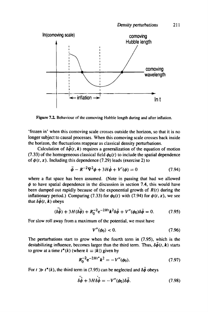
Figure 7.2. Behaviour of the comoving Hubble length during and after inflation.
'frozen in' when this comoving scale crosses outside the horizon, so that it is no
longer subject to causal processes. When this comoving scale crosses back inside
the horizon, the fluctuations reappear as classical density perturbations.
Calculation of 8~(t, k) requires a generalization of the equation of motion
(7.33) of the homogeneous classical field tPo(t) to include the spatial dependence
of t/J(t, x). Including this dependence (7.29) leads (exercise 2) to
if, - R- 2 V 2 t/J + 3HtiJ + V'(t/J) = 0
(7.94)
where a flat space has been assumed. (Note in passing that had we allowed
t/J to have spatial dependence in the discussion in section 7.4, this would have
been damped out rapidly because of the exponential growth of R(t) during the
inflationary period.) Comparing (7.33) for tPo(t) with (7.94) for t/J(t, x), we see
that 8~(t, k) obeys
(i~) + 3H (8~) + R;2e- 2Ht k28~ + V" (tPo)8~ = O.
(7.95)
For slow roll away from a maximum of the potential, we must have
V" (tPo) < O.
(7.96)
The perturbations start to grow when the fourth term in (7.95), which is the
destabilizing influence, becomes larger than the third term. Thus, 8~(t, k) starts
to grow at a time t*(k) (where k == Ikl) given by
R;2e- 2Ht Ok2 = -V"(tPo).
(7.97)
For t » ,*(k), the third term in (7.95) can be neglected and 8~ obeys
..
.
8~ + 3H 8~ = - V" (tPo)8~.
(7.98)
211
In(comoving scale)
comoving
Hubble length
ill
•
comoving
wavelength
~ inflation .....
In t
Figure 7.2. Behaviour of the comoving Hubble length during and after inflation.
'frozen in' when this comoving scale crosses outside the horizon, so that it is no
longer subject to causal processes. When this comoving scale crosses back inside
the horizon, the fluctuations reappear as classical density perturbations.
Calculation of 8~(t, k) requires a generalization of the equation of motion
(7.33) of the homogeneous classical field tPo(t) to include the spatial dependence
of t/J(t, x). Including this dependence (7.29) leads (exercise 2) to
if, - R- 2 V 2 t/J + 3HtiJ + V'(t/J) = 0
(7.94)
where a flat space has been assumed. (Note in passing that had we allowed
t/J to have spatial dependence in the discussion in section 7.4, this would have
been damped out rapidly because of the exponential growth of R(t) during the
inflationary period.) Comparing (7.33) for tPo(t) with (7.94) for t/J(t, x), we see
that 8~(t, k) obeys
(i~) + 3H (8~) + R;2e- 2Ht k28~ + V" (tPo)8~ = O.
(7.95)
For slow roll away from a maximum of the potential, we must have
V" (tPo) < O.
(7.96)
The perturbations start to grow when the fourth term in (7.95), which is the
destabilizing influence, becomes larger than the third term. Thus, 8~(t, k) starts
to grow at a time t*(k) (where k == Ikl) given by
R;2e- 2Ht Ok2 = -V"(tPo).
(7.97)
For t » ,*(k), the third term in (7.95) can be neglected and 8~ obeys
..
.
8~ + 3H 8~ = - V" (tPo)8~.
(7.98)