

455
N.1. Covariant derivatives and coordinate transformations
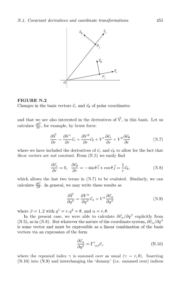
FIGURE N.2
Changes in the basis vectors → e r and → e θ of polar coordinates.
and that we are also interested in the derivatives of V → , in this basis. Let us
V
calculate
∂ → , for example, by brute force:
∂r
r
∂V →
∂V
∂V
θ
∂→ e r
∂→ e θ
r
=
→ e r +
→ e θ + V
+ V
θ
(N.7)
∂r
∂r
∂r
∂r
∂r
where we have included the derivatives of → e r and → e θ to allow for the fact that
these vectors are not constant. From (N.5) we easily find
∂→ e r
∂→ e θ
1
= 0,
= − sin θ → i + cos θ → j = → e θ ,
(N.8)
∂r
∂r
r
which allows the last two terms in (N.7) to be evaluted. Similarly, we can
V
calculate
∂ → . In general, we may write these results as
∂θ
∂V →
∂V
α
∂→ e α
=
→ e α + V
α
(N.9)
∂q β
∂q β
∂q β
1
2
where β = 1, 2 with q = r, q = θ, and α = r, θ.
In the present case, we were able to calculate ∂→ e α /∂q
β explicitly from
(N.5), as in (N.8). But whatever the nature of the coordinate system, ∂→ e α /∂q
β
is some vector and must be expressible as a linear combination of the basis
vectors via an expression of the form
∂→ e α = Γ
γ → e γ
(N.10)
αβ
∂q β
where the repeated index γ is summed over as usual (γ = r, θ). Inserting
(N.10) into (N.9) and interchanging the ‘dummy’ (i.e. summed over) indices
N.1. Covariant derivatives and coordinate transformations
FIGURE N.2
Changes in the basis vectors → e r and → e θ of polar coordinates.
and that we are also interested in the derivatives of V → , in this basis. Let us
V
calculate
∂ → , for example, by brute force:
∂r
r
∂V →
∂V
∂V
θ
∂→ e r
∂→ e θ
r
=
→ e r +
→ e θ + V
+ V
θ
(N.7)
∂r
∂r
∂r
∂r
∂r
where we have included the derivatives of → e r and → e θ to allow for the fact that
these vectors are not constant. From (N.5) we easily find
∂→ e r
∂→ e θ
1
= 0,
= − sin θ → i + cos θ → j = → e θ ,
(N.8)
∂r
∂r
r
which allows the last two terms in (N.7) to be evaluted. Similarly, we can
V
calculate
∂ → . In general, we may write these results as
∂θ
∂V →
∂V
α
∂→ e α
=
→ e α + V
α
(N.9)
∂q β
∂q β
∂q β
1
2
where β = 1, 2 with q = r, q = θ, and α = r, θ.
In the present case, we were able to calculate ∂→ e α /∂q
β explicitly from
(N.5), as in (N.8). But whatever the nature of the coordinate system, ∂→ e α /∂q
β
is some vector and must be expressible as a linear combination of the basis
vectors via an expression of the form
∂→ e α = Γ
γ → e γ
(N.10)
αβ
∂q β
where the repeated index γ is summed over as usual (γ = r, θ). Inserting
(N.10) into (N.9) and interchanging the ‘dummy’ (i.e. summed over) indices