

454
N. Geometrical Aspects of Gauge Fields
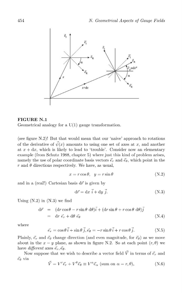
FIGURE N.1
Geometrical analogy for a U(1) gauge transformation.
(see figure N.2)! But that would mean that our ‘naive’ approach to rotations
of the derivative of ψ → (x) amounts to using one set of axes at x, and another
at x + dx, which is likely to lead to ‘trouble’. Consider now an elementary
example (from Schutz 1988, chapter 5) where just this kind of problem arises,
namely the use of polar coordinate basis vectors → e r and → e θ , which point in the
r and θ directions respectively. We have, as usual,
x = r cos θ, y = r sin θ
(N.2)
and in a (real!) Cartesian basis d→ r is given by
d→ r = dx → i + dy → j.
(N.3)
Using (N.2) in (N.3) we find
d→ r = (dr cos θ − r sin θ dθ) → i + (dr sin θ + r cos θ dθ) → j
= dr → e r + dθ → e θ
(N.4)
where
→ e r = cos θ → i + sin θ → j, → e θ = −r sin θ → i + r cos θ → j.
(N.5)
Plainly, → e r and → e θ change direction (and even magnitude, for → e θ ) as we move
about in the x − y plane, as shown in figure N.2. So at each point (r, θ) we
have different axes → e r , → e θ .
Now suppose that we wish to describe a vector field V → in terms of → e r and
→ e θ via
→
r → e r + V
θ → e θ ≡ V
α →
V = V
e α (sum on α = r, θ),
(N.6)
N. Geometrical Aspects of Gauge Fields
FIGURE N.1
Geometrical analogy for a U(1) gauge transformation.
(see figure N.2)! But that would mean that our ‘naive’ approach to rotations
of the derivative of ψ → (x) amounts to using one set of axes at x, and another
at x + dx, which is likely to lead to ‘trouble’. Consider now an elementary
example (from Schutz 1988, chapter 5) where just this kind of problem arises,
namely the use of polar coordinate basis vectors → e r and → e θ , which point in the
r and θ directions respectively. We have, as usual,
x = r cos θ, y = r sin θ
(N.2)
and in a (real!) Cartesian basis d→ r is given by
d→ r = dx → i + dy → j.
(N.3)
Using (N.2) in (N.3) we find
d→ r = (dr cos θ − r sin θ dθ) → i + (dr sin θ + r cos θ dθ) → j
= dr → e r + dθ → e θ
(N.4)
where
→ e r = cos θ → i + sin θ → j, → e θ = −r sin θ → i + r cos θ → j.
(N.5)
Plainly, → e r and → e θ change direction (and even magnitude, for → e θ ) as we move
about in the x − y plane, as shown in figure N.2. So at each point (r, θ) we
have different axes → e r , → e θ .
Now suppose that we wish to describe a vector field V → in terms of → e r and
→ e θ via
→
r → e r + V
θ → e θ ≡ V
α →
V = V
e α (sum on α = r, θ),
(N.6)