

441
M.4. Examples
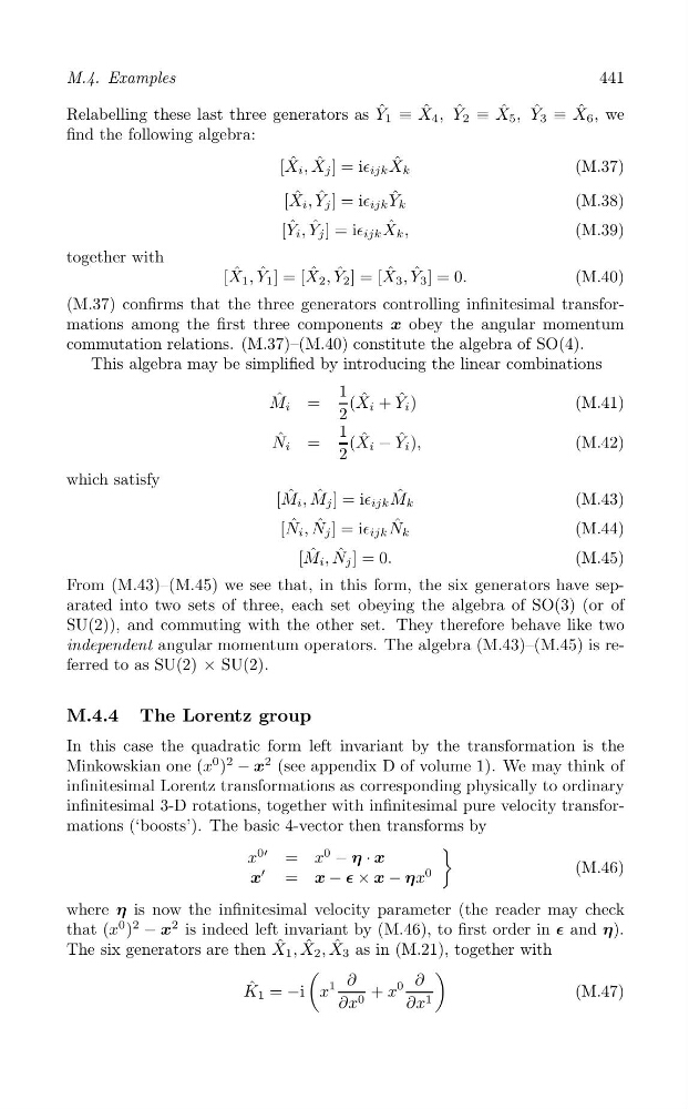
Relabelling these last three generators as Y ˆ 1 ≡ X ˆ 4 , Y ˆ 2 ≡ X ˆ 5 , Y ˆ 3 ≡ X ˆ 6 , we
find the following algebra:
[X ˆ i , X ˆ j ] = i∈ ijk X ˆ k
(M.37)
[X ˆ i , Y ˆ j ] = i∈ ijk Y ˆ k
(M.38)
[Y ˆ i , Y ˆ j ] = i∈ ijk X ˆ k ,
(M.39)
together with
[X ˆ 1 , Y ˆ 1 ] = [ X ˆ 2 , Y ˆ 2 ] = [ X ˆ 3 , Y ˆ 3 ] = 0.
(M.40)
(M.37) confirms that the three generators controlling infinitesimal transformations among the first three components x obey the angular momentum
commutation relations. (M.37)–(M.40) constitute the algebra of SO(4).
This algebra may be simplified by introducing the linear combinations
ˆ
M i =
1 (X ˆ i + Y ˆ i )
(M.41)
2
ˆ
N i =
1 (X ˆ i − Y ˆ i ),
(M.42)
2
which satisfy
ˆ
ˆ
[M ˆ i , M j ] = i∈ ijk M k
(M.43)
[N ˆ i , N ˆ j ] = i∈ ijk N ˆ k
(M.44)
[M ˆ i , N ˆ j ] = 0.
(M.45)
From (M.43)–(M.45) we see that, in this form, the six generators have separated into two sets of three, each set obeying the algebra of SO(3) (or of
SU(2)), and commuting with the other set. They therefore behave like two
independent angular momentum operators. The algebra (M.43)–(M.45) is referred to as SU(2) × SU(2).
M.4.4 The Lorentz group
In this case the quadratic form left invariant by the transformation is the
Minkowskian one (x
0 )
2
− x
2 (see appendix D of volume 1). We may think of
infinitesimal Lorentz transformations as corresponding physically to ordinary
infinitesimal 3-D rotations, together with infinitesimal pure velocity transformations (‘boosts’). The basic 4-vector then transforms by
)
x
0′
= x
0
− η · x
(M.46)
′
0
x = x − ∊ × x − ηx
where η is now the infinitesimal velocity parameter (the reader may check
2
that (x
0 )
2
− x is indeed left invariant by (M.46), to first order in ∊ and η).
The six generators are then X ˆ 1 , X ˆ 2 , X ˆ 3 as in (M.21), together with
(
)
∂
∂
1
0
ˆ
K 1 = −i x
+ x
(M.47)
∂x 0
∂x 1
M.4. Examples
Relabelling these last three generators as Y ˆ 1 ≡ X ˆ 4 , Y ˆ 2 ≡ X ˆ 5 , Y ˆ 3 ≡ X ˆ 6 , we
find the following algebra:
[X ˆ i , X ˆ j ] = i∈ ijk X ˆ k
(M.37)
[X ˆ i , Y ˆ j ] = i∈ ijk Y ˆ k
(M.38)
[Y ˆ i , Y ˆ j ] = i∈ ijk X ˆ k ,
(M.39)
together with
[X ˆ 1 , Y ˆ 1 ] = [ X ˆ 2 , Y ˆ 2 ] = [ X ˆ 3 , Y ˆ 3 ] = 0.
(M.40)
(M.37) confirms that the three generators controlling infinitesimal transformations among the first three components x obey the angular momentum
commutation relations. (M.37)–(M.40) constitute the algebra of SO(4).
This algebra may be simplified by introducing the linear combinations
ˆ
M i =
1 (X ˆ i + Y ˆ i )
(M.41)
2
ˆ
N i =
1 (X ˆ i − Y ˆ i ),
(M.42)
2
which satisfy
ˆ
ˆ
[M ˆ i , M j ] = i∈ ijk M k
(M.43)
[N ˆ i , N ˆ j ] = i∈ ijk N ˆ k
(M.44)
[M ˆ i , N ˆ j ] = 0.
(M.45)
From (M.43)–(M.45) we see that, in this form, the six generators have separated into two sets of three, each set obeying the algebra of SO(3) (or of
SU(2)), and commuting with the other set. They therefore behave like two
independent angular momentum operators. The algebra (M.43)–(M.45) is referred to as SU(2) × SU(2).
M.4.4 The Lorentz group
In this case the quadratic form left invariant by the transformation is the
Minkowskian one (x
0 )
2
− x
2 (see appendix D of volume 1). We may think of
infinitesimal Lorentz transformations as corresponding physically to ordinary
infinitesimal 3-D rotations, together with infinitesimal pure velocity transformations (‘boosts’). The basic 4-vector then transforms by
)
x
0′
= x
0
− η · x
(M.46)
′
0
x = x − ∊ × x − ηx
where η is now the infinitesimal velocity parameter (the reader may check
2
that (x
0 )
2
− x is indeed left invariant by (M.46), to first order in ∊ and η).
The six generators are then X ˆ 1 , X ˆ 2 , X ˆ 3 as in (M.21), together with
(
)
∂
∂
1
0
ˆ
K 1 = −i x
+ x
(M.47)
∂x 0
∂x 1