

68
3. Relativistic Quantum Mechanics
linear combination (always allowed for degenerate states) we can write these
wavefunctions as (x, y, z)f (r), where again a normalization factor has been
omitted. In this form it is plain that the multiplicity of the p-state wavefunctions can be interpreted in simple geometrical terms: they are effectively the
components of a vector (multiplication by the scalar function f (r) does not
affect this).
The several components of the Dirac wavefunction together make up a
similar, but quite distinct, object called a spinor. We shall have more to say
about this in chapter 4. For the moment we continue with the problem of
finding the matrices α i and β to satisfy (3.28)–(3.30).
As problem 3.2 shows, the smallest possible dimension of the matrices for
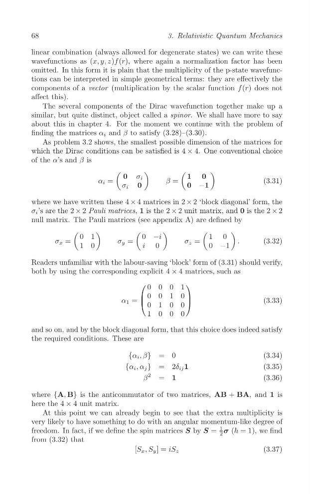
which the Dirac conditions can be satisfied is 4 × 4. One conventional choice
of the α’s and β is
(
)
(
)
0 σ i
1 0
α i =
β =
(3.31)
σ i 0
0 −1
where we have written these 4 × 4 matrices in 2 × 2 ‘block diagonal’ form, the
σ i ’s are the 2 × 2 Pauli matrices, 1 is the 2 × 2 unit matrix, and 0 is the 2 × 2
null matrix. The Pauli matrices (see appendix A) are defined by
(
)
(
)
(
)
0 1
0 −i
1 0
σ x =
σ y =
σ z =
.
(3.32)
1 0
i 0
0 −1
Readers unfamiliar with the labour-saving ‘block’ form of (3.31) should verify,
both by using the corresponding explicit 4 × 4 matrices, such as
(
)
0 0 0 1
| 0 0 1 0|
α 1 = (
)
(3.33)
0 1 0 0
1 0 0 0
and so on, and by the block diagonal form, that this choice does indeed satisfy
the required conditions. These are
{α i , β} = 0
(3.34)
{α i , α j } = 2δ ij 1
(3.35)
β
2
= 1
(3.36)
where {A, B} is the anticommutator of two matrices, AB + BA, and 1 is
here the 4 × 4 unit matrix.
At this point we can already begin to see that the extra multiplicity is
very likely to have something to do with an angular momentum-like degree of
1
freedom. In fact, if we define the spin matrices S by S = σ (ħ = 1), we find
2
from (3.32) that
[S x , S y ] = iS z
(3.37)
3. Relativistic Quantum Mechanics
linear combination (always allowed for degenerate states) we can write these
wavefunctions as (x, y, z)f (r), where again a normalization factor has been
omitted. In this form it is plain that the multiplicity of the p-state wavefunctions can be interpreted in simple geometrical terms: they are effectively the
components of a vector (multiplication by the scalar function f (r) does not
affect this).
The several components of the Dirac wavefunction together make up a
similar, but quite distinct, object called a spinor. We shall have more to say
about this in chapter 4. For the moment we continue with the problem of
finding the matrices α i and β to satisfy (3.28)–(3.30).
As problem 3.2 shows, the smallest possible dimension of the matrices for
which the Dirac conditions can be satisfied is 4 × 4. One conventional choice
of the α’s and β is
(
)
(
)
0 σ i
1 0
α i =
β =
(3.31)
σ i 0
0 −1
where we have written these 4 × 4 matrices in 2 × 2 ‘block diagonal’ form, the
σ i ’s are the 2 × 2 Pauli matrices, 1 is the 2 × 2 unit matrix, and 0 is the 2 × 2
null matrix. The Pauli matrices (see appendix A) are defined by
(
)
(
)
(
)
0 1
0 −i
1 0
σ x =
σ y =
σ z =
.
(3.32)
1 0
i 0
0 −1
Readers unfamiliar with the labour-saving ‘block’ form of (3.31) should verify,
both by using the corresponding explicit 4 × 4 matrices, such as
(
)
0 0 0 1
| 0 0 1 0|
α 1 = (
)
(3.33)
0 1 0 0
1 0 0 0
and so on, and by the block diagonal form, that this choice does indeed satisfy
the required conditions. These are
{α i , β} = 0
(3.34)
{α i , α j } = 2δ ij 1
(3.35)
β
2
= 1
(3.36)
where {A, B} is the anticommutator of two matrices, AB + BA, and 1 is
here the 4 × 4 unit matrix.
At this point we can already begin to see that the extra multiplicity is
very likely to have something to do with an angular momentum-like degree of
1
freedom. In fact, if we define the spin matrices S by S = σ (ħ = 1), we find
2
from (3.32) that
[S x , S y ] = iS z
(3.37)