

66
3. Relativistic Quantum Mechanics
3.2 The Dirac equation
In the case of the KG equation it is clear why the problem arose:
(i) In constructing a wave equation in close correspondence with the
squared energy–momentum relation
2
2
E
2 = p + m
we immediately allowed negative-energy solutions.
(ii) The KG equation has a ∂
2 /∂t
2 term: this leads to a continuity
equation with a ‘probability density’ containing ∂/∂t, and hence to
negative probabilities.
Dirac approached these problems in his characteristically direct way. In
order to obtain a positive-definite probability density ρ ≥ 0, he required an
equation linear in ∂/∂t. Then, for relativistic covariance (see chapter 4), the
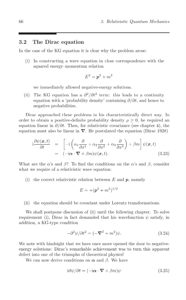
equation must also be linear in ∇. He postulated the equation (Dirac 1928)
[ (
)
]
∂ψ(x, t)
∂
∂
∂
i
=
−i α 1
+ α 2
+ α 3
+ βm ψ(x, t)
∂t
∂x 1
∂x 2
∂x 3
= (−iα · ∇ + βm)ψ(x, t).
(3.23)
What are the α’s and β? To find the conditions on the α’s and β, consider
what we require of a relativistic wave equation:
(i) the correct relativistic relation between E and p, namely
2
2 )
1/2
E = +(p + m
(ii) the equation should be covariant under Lorentz transformations.
We shall postpone discussion of (ii) until the following chapter. To solve
requirement (i), Dirac in fact demanded that his wavefunction ψ satisfy, in
addition, a KG-type condition
−∂
2 ψ/∂t
2 = (−∇
2 + m
2 )ψ.
(3.24)
We note with hindsight that we have once more opened the door to negativeenergy solutions: Dirac’s remarkable achievement was to turn this apparent
defect into one of the triumphs of theoretical physics!
We can now derive conditions on α and β. We have
i∂ψ/∂t = (−iα · ∇ + βm)ψ
(3.25)
3. Relativistic Quantum Mechanics
3.2 The Dirac equation
In the case of the KG equation it is clear why the problem arose:
(i) In constructing a wave equation in close correspondence with the
squared energy–momentum relation
2
2
E
2 = p + m
we immediately allowed negative-energy solutions.
(ii) The KG equation has a ∂
2 /∂t
2 term: this leads to a continuity
equation with a ‘probability density’ containing ∂/∂t, and hence to
negative probabilities.
Dirac approached these problems in his characteristically direct way. In
order to obtain a positive-definite probability density ρ ≥ 0, he required an
equation linear in ∂/∂t. Then, for relativistic covariance (see chapter 4), the
equation must also be linear in ∇. He postulated the equation (Dirac 1928)
[ (
)
]
∂ψ(x, t)
∂
∂
∂
i
=
−i α 1
+ α 2
+ α 3
+ βm ψ(x, t)
∂t
∂x 1
∂x 2
∂x 3
= (−iα · ∇ + βm)ψ(x, t).
(3.23)
What are the α’s and β? To find the conditions on the α’s and β, consider
what we require of a relativistic wave equation:
(i) the correct relativistic relation between E and p, namely
2
2 )
1/2
E = +(p + m
(ii) the equation should be covariant under Lorentz transformations.
We shall postpone discussion of (ii) until the following chapter. To solve
requirement (i), Dirac in fact demanded that his wavefunction ψ satisfy, in
addition, a KG-type condition
−∂
2 ψ/∂t
2 = (−∇
2 + m
2 )ψ.
(3.24)
We note with hindsight that we have once more opened the door to negativeenergy solutions: Dirac’s remarkable achievement was to turn this apparent
defect into one of the triumphs of theoretical physics!
We can now derive conditions on α and β. We have
i∂ψ/∂t = (−iα · ∇ + βm)ψ
(3.25)