

311
20.7. Quark weak currents
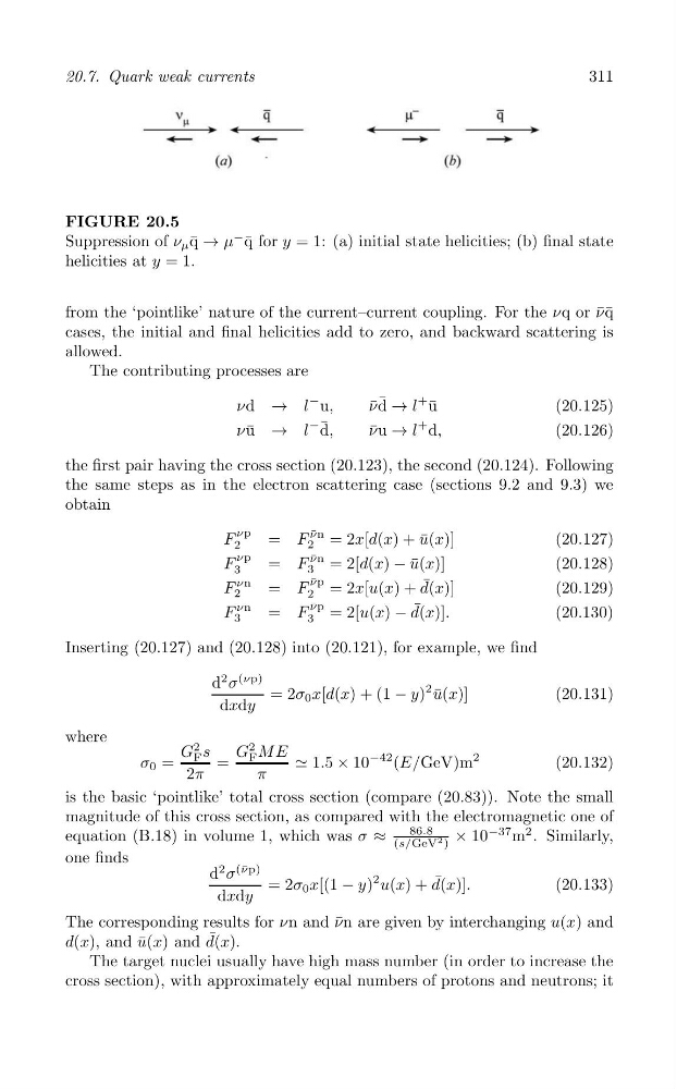
FIGURE 20.5
Suppression of ν μ q ¯ → μ
− ¯
=
q for y 1: (a) initial state helicities; (b) final state
helicities at y = 1.
from the ‘pointlike’ nature of the current–current coupling. For the νq or ¯
νq ¯
cases, the initial and final helicities add to zero, and backward scattering is
allowed.
The contributing processes are
νd → l
− u,
ν ¯d ¯ → l
+ u ¯
(20.125)
νu ¯ → l
− d ¯ ,
ν ¯u → l
+ d,
(20.126)
the first pair having the cross section (20.123), the second (20.124). Following
the same steps as in the electron scattering case (sections 9.2 and 9.3) we
obtain
νp
ν ¯n
F
= F = 2x[d(x) + u ¯(x)]
(20.127)
2
2
νp
ν ¯n
F
= F = 2[d(x) − u ¯(x)]
(20.128)
3
3
F
νn
= F
ν ¯p = 2x[u(x) + d ¯ (x)]
(20.129)
2
2
F
νn
ν ¯p
= F = 2[u(x) − d ¯ (x)].
(20.130)
3
3
Inserting (20.127) and (20.128) into (20.121), for example, we find
d
2 σ
(νp)
= 2σ 0 x[d(x) + (1 − y)
2 u ¯(x)]
(20.131)
dxdy
where
G
2
G
2
F s
M E
F
σ 0 =
=
⋍ 1.5 × 10
−42 (E/GeV)m
2
(20.132)
2π
π
is the basic ‘pointlike’ total cross section (compare (20.83)). Note the small
magnitude of this cross section, as compared with the electromagnetic one of
86.8
× 10
−37
equation (B.18) in volume 1, which was σ ≈
m
2 . Similarly,
(s/GeV 2 )
one finds
d
2 σ
(¯ νp)
= 2σ 0 x[(1 − y)
2 u(x) + d ¯ (x)].
(20.133)
dxdy
The corresponding results for νn and ¯
νn are given by interchanging u(x) and
d(x), and ¯
u(x) and d ¯ (x).
The target nuclei usually have high mass number (in order to increase the
cross section), with approximately equal numbers of protons and neutrons; it