

62
2.1
2. Electromagnetism as a Gauge Theory
Problems
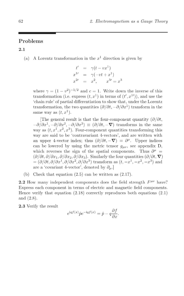
(a) A Lorentz transformation in the x
1 direction is given by
′
t = γ(t − vx
1 )
1′
x
= γ(−vt + x
1 )
2′
2
3′
3
x
= x ,
x = x
2 )
−1/2
where γ = (1 − v
and c = 1. Write down the inverse of this
transformation (i.e. express (t, x
1 ) in terms of (t
′ , x
1′ )), and use the
‘chain rule’ of partial differentiation to show that, under the Lorentz
transformation, the two quantities (∂/∂t, −∂/∂x
1 ) transform in the
same way as (t, x
1 ).
[The general result is that the four-component quantity (∂/∂t,
−∂/∂x
1 , −∂/∂x
2 , −∂/∂x
3 ) ≡ (∂/∂t, −∇) transforms in the same
2
way as (t, x
1 , x , x
3 ). Four-component quantities transforming this
way are said to be ‘contravariant 4-vectors’, and are written with
an upper 4-vector index; thus (∂/∂t, −∇) ≡ ∂
μ . Upper indices
can be lowered by using the metric tensor g μν , see appendix D,
which reverses the sign of the spatial components. Thus ∂
μ =
(∂/∂t, ∂/∂x 1 , ∂/∂x 2 , ∂/∂x 3 ). Similarly the four quantities (∂/∂t, ∇)
1
2
= (∂/∂t, ∂/∂x
1 , ∂/∂x
2 , ∂/∂x
3 ) transform as (t, −x , −x , −x
3 ) and
are a ‘covariant 4-vector’, denoted by ∂ μ .]
(b) Check that equation (2.5) can be written as (2.17).
2.2 How many independent components does the field strength F
μν have?
Express each component in terms of electric and magnetic field components.
Hence verify that equation (2.18) correctly reproduces both equations (2.1)
and (2.8).
2.3 Verify the result
iqf (x) ˆ
e
pe
−iqf (x) = ˆ
p − q
∂f .
∂x
2.1
2. Electromagnetism as a Gauge Theory
Problems
(a) A Lorentz transformation in the x
1 direction is given by
′
t = γ(t − vx
1 )
1′
x
= γ(−vt + x
1 )
2′
2
3′
3
x
= x ,
x = x
2 )
−1/2
where γ = (1 − v
and c = 1. Write down the inverse of this
transformation (i.e. express (t, x
1 ) in terms of (t
′ , x
1′ )), and use the
‘chain rule’ of partial differentiation to show that, under the Lorentz
transformation, the two quantities (∂/∂t, −∂/∂x
1 ) transform in the
same way as (t, x
1 ).
[The general result is that the four-component quantity (∂/∂t,
−∂/∂x
1 , −∂/∂x
2 , −∂/∂x
3 ) ≡ (∂/∂t, −∇) transforms in the same
2
way as (t, x
1 , x , x
3 ). Four-component quantities transforming this
way are said to be ‘contravariant 4-vectors’, and are written with
an upper 4-vector index; thus (∂/∂t, −∇) ≡ ∂
μ . Upper indices
can be lowered by using the metric tensor g μν , see appendix D,
which reverses the sign of the spatial components. Thus ∂
μ =
(∂/∂t, ∂/∂x 1 , ∂/∂x 2 , ∂/∂x 3 ). Similarly the four quantities (∂/∂t, ∇)
1
2
= (∂/∂t, ∂/∂x
1 , ∂/∂x
2 , ∂/∂x
3 ) transform as (t, −x , −x , −x
3 ) and
are a ‘covariant 4-vector’, denoted by ∂ μ .]
(b) Check that equation (2.5) can be written as (2.17).
2.2 How many independent components does the field strength F
μν have?
Express each component in terms of electric and magnetic field components.
Hence verify that equation (2.18) correctly reproduces both equations (2.1)
and (2.8).
2.3 Verify the result
iqf (x) ˆ
e
pe
−iqf (x) = ˆ
p − q
∂f .
∂x