

60
2. Electromagnetism as a Gauge Theory
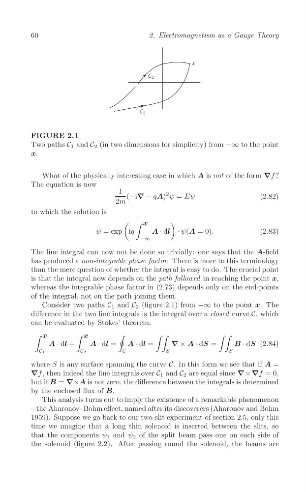
FIGURE 2.1
Two paths C 1 and C 2 (in two dimensions for simplicity) from −∞ to the point
x.
What of the physically interesting case in which A is not of the form ∇f ?
The equation is now
1
2m
(−i∇ − qA)
2 ψ = Eψ
(2.82)
to which the solution is
ψ = exp
(
iq
∫ x
−∞
A · dl
)
· ψ(A = 0).
(2.83)
The line integral can now not be done so trivially: one says that the A-field
has produced a non-integrable phase factor. There is more to this terminology
than the mere question of whether the integral is easy to do. The crucial point
is that the integral now depends on the path followed in reaching the point x,
whereas the integrable phase factor in (2.73) depends only on the end-points
of the integral, not on the path joining them.
Consider two paths C 1 and C 2 (figure 2.1) from −∞ to the point x. The
difference in the two line integrals is the integral over a closed curve C, which
can be evaluated by Stokes’ theorem:
∫
∫
∮
∫ ∫
∫ ∫
x
x
A · dl −
A · dl =
A · dl =
∇ × A · dS =
B · dS (2.84)
C1
C2
C
S
S
where S is any surface spanning the curve C. In this form we see that if A =
∇f , then indeed the line integrals over C 1 and C 2 are equal since ∇ × ∇f = 0,
but if B = ∇×A is not zero, the difference between the integrals is determined
by the enclosed flux of B.
This analysis turns out to imply the existence of a remarkable phenomenon
– the Aharonov–Bohm effect, named after its discoverers (Aharonov and Bohm
1959). Suppose we go back to our two-slit experiment of section 2.5, only this
time we imagine that a long thin solenoid is inserted between the slits, so
that the components ψ 1 and ψ 2 of the split beam pass one on each side of
the solenoid (figure 2.2). After passing round the solenoid, the beams are
2. Electromagnetism as a Gauge Theory
FIGURE 2.1
Two paths C 1 and C 2 (in two dimensions for simplicity) from −∞ to the point
x.
What of the physically interesting case in which A is not of the form ∇f ?
The equation is now
1
2m
(−i∇ − qA)
2 ψ = Eψ
(2.82)
to which the solution is
ψ = exp
(
iq
∫ x
−∞
A · dl
)
· ψ(A = 0).
(2.83)
The line integral can now not be done so trivially: one says that the A-field
has produced a non-integrable phase factor. There is more to this terminology
than the mere question of whether the integral is easy to do. The crucial point
is that the integral now depends on the path followed in reaching the point x,
whereas the integrable phase factor in (2.73) depends only on the end-points
of the integral, not on the path joining them.
Consider two paths C 1 and C 2 (figure 2.1) from −∞ to the point x. The
difference in the two line integrals is the integral over a closed curve C, which
can be evaluated by Stokes’ theorem:
∫
∫
∮
∫ ∫
∫ ∫
x
x
A · dl −
A · dl =
A · dl =
∇ × A · dS =
B · dS (2.84)
C1
C2
C
S
S
where S is any surface spanning the curve C. In this form we see that if A =
∇f , then indeed the line integrals over C 1 and C 2 are equal since ∇ × ∇f = 0,
but if B = ∇×A is not zero, the difference between the integrals is determined
by the enclosed flux of B.
This analysis turns out to imply the existence of a remarkable phenomenon
– the Aharonov–Bohm effect, named after its discoverers (Aharonov and Bohm
1959). Suppose we go back to our two-slit experiment of section 2.5, only this
time we imagine that a long thin solenoid is inserted between the slits, so
that the components ψ 1 and ψ 2 of the split beam pass one on each side of
the solenoid (figure 2.2). After passing round the solenoid, the beams are