

277
19.6. Spontaneously broken local SU(2) × U(1) symmetry
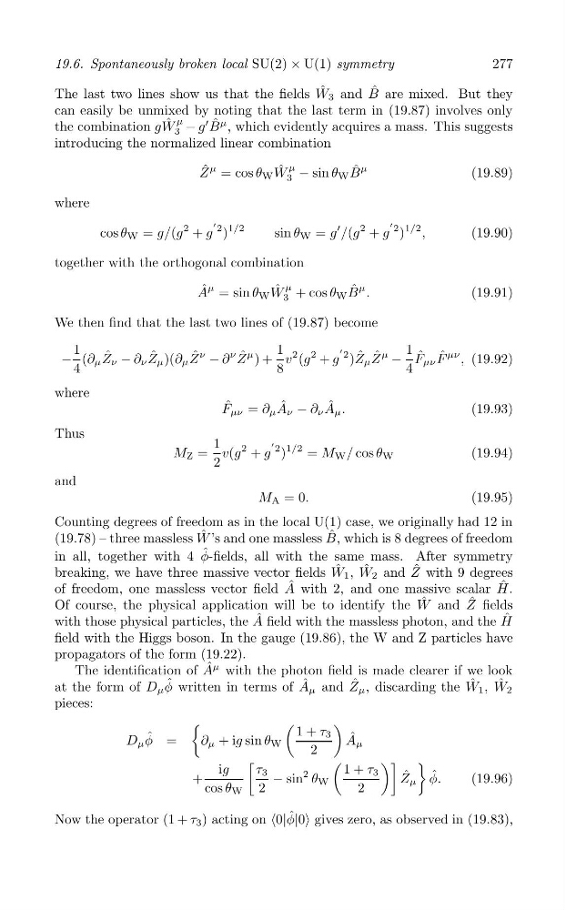
The last two lines show us that the fields W ˆ 3 and B ˆ are mixed. But they
can easily be unmixed by noting that the last term in (19.87) involves only
μ
′
the combination gW ˆ − g B ˆ μ , which evidently acquires a mass. This suggests
3
introducing the normalized linear combination
Z ˆ μ
W ˆ μ
B ˆ μ
= cos θ W 3 − sin θ W
(19.89)
where
2
2 )
1/2
2
cos θ W = g/(g + g
′
sin θ W = g
′ /(g + g
′ 2 )
1/2 ,
(19.90)
together with the orthogonal combination
μ
A ˆ μ = sin θ W W ˆ + cos θ W B ˆ μ .
(19.91)
3
We then find that the last two lines of (19.87) become
1
ˆ
ˆ
ˆ
1
2
2 ) ˆ ˆ
1 ˆ F ˆ μν
− (∂ μ Z ν − ∂ ν Z μ )(∂ μ Z
ν
− ∂
ν Z ˆ μ ) + v
2 (g + g
′
Z μ Z
μ
− F μν
, (19.92)
4
8
4
where
ˆ
ˆ
ˆ
F μν = ∂ μ A ν − ∂ ν A μ .
(19.93)
Thus
′
1
2
2 )
1/2
M Z = v(g + g
= M W / cos θ W
(19.94)
2
and
M A = 0.
(19.95)
Counting degrees of freedom as in the local U(1) case, we originally had 12 in
(19.78) – three massless W ˆ ’s and one massless B ˆ , which is 8 degrees of freedom
in all, together with 4 φ ˆ -fields, all with the same mass. After symmetry
breaking, we have three massive vector fields W ˆ 1 , W ˆ 2 and Z ˆ with 9 degrees
of freedom, one massless vector field A ˆ with 2, and one massive scalar H ˆ .
Of course, the physical application will be to identify the W ˆ and Z ˆ fields
with those physical particles, the A ˆ field with the massless photon, and the H ˆ
field with the Higgs boson. In the gauge (19.86), the W and Z particles have
propagators of the form (19.22).
The identification of A ˆ μ with the photon field is made clearer if we look
at the form of D μ φ ˆ written in terms of A ˆ μ and Z ˆ μ , discarding the W ˆ 1 , W ˆ 2
pieces:
(
(
)
1 + τ 3
ˆ
ˆ
D μ φ =
∂ μ + ig sin θ W
A μ
2
[
(
)] )
ig
τ 3
1 + τ 3
ˆ
ˆ
+
− sin
2 θ W
Z μ φ.
(19.96)
cos θ W 2
2
Now the operator (1 + τ 3 ) acting on ‹0|φ ˆ |0› gives zero, as observed in (19.83),