

273
19.5. ’t Hooft’s gauges
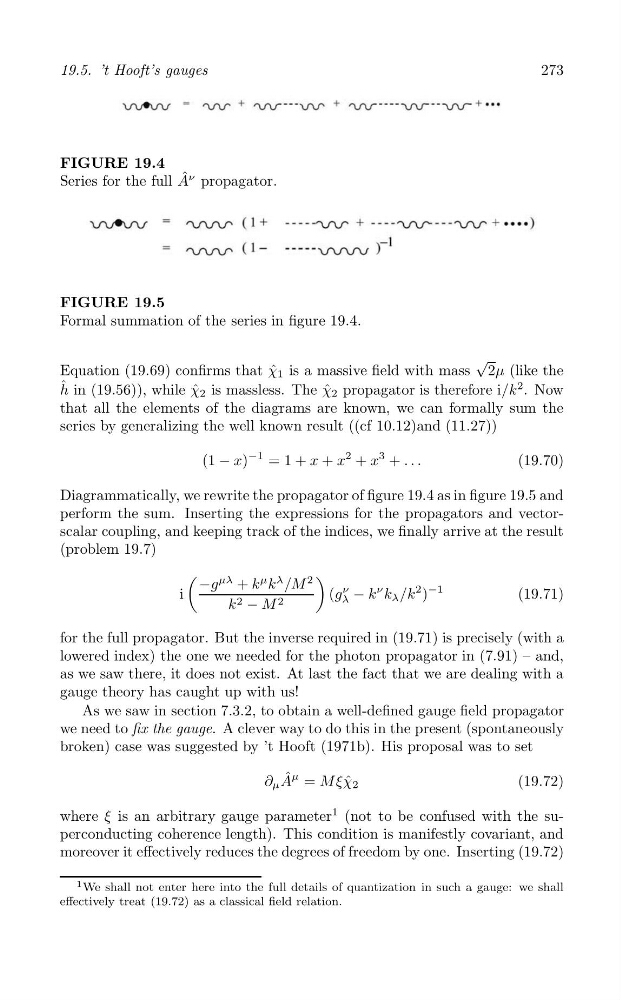
FIGURE 19.4
Series for the full A ˆ ν propagator.
FIGURE 19.5
Formal summation of the series in figure 19.4.
√
Equation (19.69) confirms that ˆ
χ 1 is a massive field with mass 2μ (like the
h ˆ in (19.56)), while ˆ
χ 2 is massless. The ˆ
χ 2 propagator is therefore i/k
2 . Now
that all the elements of the diagrams are known, we can formally sum the
series by generalizing the well known result ((cf 10.12)and (11.27))
2
3
(1 − x)
−1 = 1 + x + x + x + . . .
(19.70)
Diagrammatically, we rewrite the propagator of figure 19.4 as in figure 19.5 and
perform the sum. Inserting the expressions for the propagators and vectorscalar coupling, and keeping track of the indices, we finally arrive at the result
(problem 19.7)
(
)
μλ
−g + k
μ k
λ /M
2
ν
i
(g λ − k
ν k λ /k
2 )
−1
(19.71)
k 2 − M 2
for the full propagator. But the inverse required in (19.71) is precisely (with a
lowered index) the one we needed for the photon propagator in (7.91) – and,
as we saw there, it does not exist. At last the fact that we are dealing with a
gauge theory has caught up with us!
As we saw in section 7.3.2, to obtain a well-defined gauge field propagator
we need to fix the gauge. A clever way to do this in the present (spontaneously
broken) case was suggested by ’t Hooft (1971b). His proposal was to set
A ˆ μ
∂ μ
= M ξχ ˆ 2
(19.72)
where ξ is an arbitrary gauge parameter
1 (not to be confused with the superconducting coherence length). This condition is manifestly covariant, and
moreover it effectively reduces the degrees of freedom by one. Inserting (19.72)
1 We shall not enter here into the full details of quantization in such a gauge: we shall
effectively treat (19.72) as a classical field relation.