

272
19. Spontaneously Broken Local Symmetry
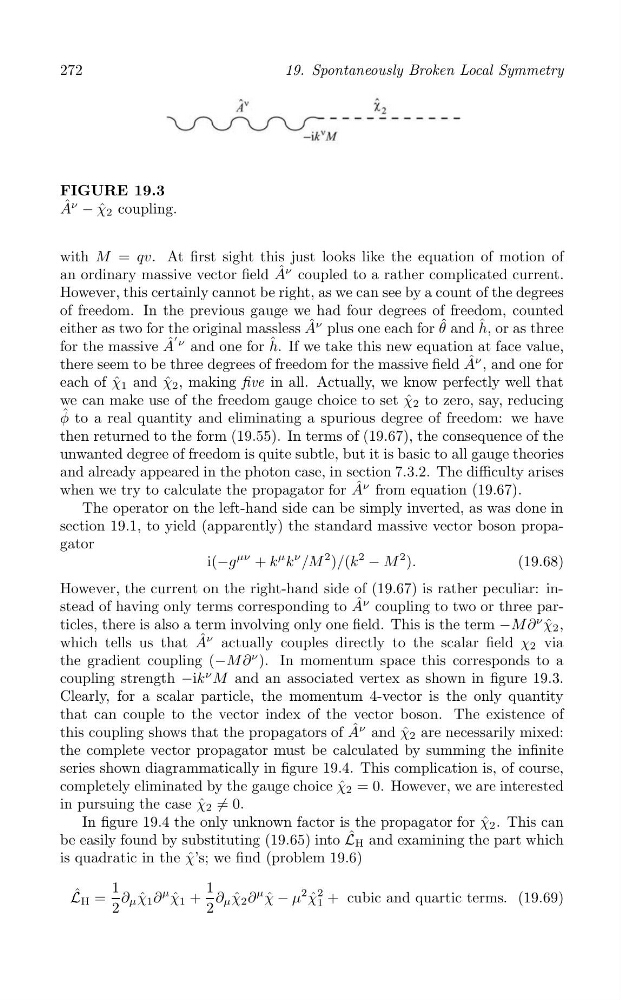
FIGURE 19.3
A ˆ ν − ˆ
χ 2 coupling.
with M = qv. At first sight this just looks like the equation of motion of
an ordinary massive vector field A ˆ ν coupled to a rather complicated current.
However, this certainly cannot be right, as we can see by a count of the degrees
of freedom. In the previous gauge we had four degrees of freedom, counted
either as two for the original massless A ˆ ν plus one each for θ ˆ and h ˆ , or as three
ν
for the massive A ˆ
′
and one for h ˆ . If we take this new equation at face value,
there seem to be three degrees of freedom for the massive field A ˆ ν , and one for
each of ˆ
χ 1 and ˆ
χ 2 , making five in all. Actually, we know perfectly well that
we can make use of the freedom gauge choice to set ˆ
χ 2 to zero, say, reducing
ˆ
φ to a real quantity and eliminating a spurious degree of freedom: we have
then returned to the form (19.55). In terms of (19.67), the consequence of the
unwanted degree of freedom is quite subtle, but it is basic to all gauge theories
and already appeared in the photon case, in section 7.3.2. The difficulty arises
when we try to calculate the propagator for A ˆ ν from equation (19.67).
The operator on the left-hand side can be simply inverted, as was done in
section 19.1, to yield (apparently) the standard massive vector boson propagator
μν
i(−g + k
μ k
ν /M
2 )/(k
2
− M
2 ).
(19.68)
However, the current on the right-hand side of (19.67) is rather peculiar: instead of having only terms corresponding to A ˆ ν coupling to two or three particles, there is also a term involving only one field. This is the term −M ∂
ν χ ˆ 2 ,
which tells us that A ˆ ν actually couples directly to the scalar field χ 2 via
the gradient coupling (−M ∂
ν ). In momentum space this corresponds to a
coupling strength −ik
ν M and an associated vertex as shown in figure 19.3.
Clearly, for a scalar particle, the momentum 4-vector is the only quantity
that can couple to the vector index of the vector boson. The existence of
this coupling shows that the propagators of A ˆ ν and ˆ
χ 2 are necessarily mixed:
the complete vector propagator must be calculated by summing the infinite
series shown diagrammatically in figure 19.4. This complication is, of course,
completely eliminated by the gauge choice ˆ
χ 2 = 0. However, we are interested
in pursuing the case ˆ
χ 2 = 0.
/
In figure 19.4 the only unknown factor is the propagator for ˆ
χ 2 . This can
be easily found by substituting (19.65) into L ˆ H and examining the part which
is quadratic in the ˆ
χ’s; we find (problem 19.6)
L ˆ H =
1 ∂ μ χ ˆ 1 ∂
μ χ ˆ 1 +
1 ∂ μ χ ˆ 2 ∂
μ χ ˆ − μ
2 χ ˆ
2
1 + cubic and quartic terms. (19.69)
2
2