

241
18.3. Effective Lagrangians
where
η = (∊ R − ∊ L )/2, ∊ = (∊ R + ∊ L )/2.
(18.78)
Evidently ∊ R = η + ∊ and ∊ L = ∊ − η, which we may compare with the L and
R transformation of the quark fields in (18.37), (18.38).
With the sign of μ
2 as in (18.73), the classical potential has a minimum at
π
2
2
σ ˆ
2 + ˆ = 4μ
2 /λ ≡ v ,
(18.79)
which we interpret as the symmetry breaking condition
2
‹0|σ ˆ
2 + π ˆ
2 |0› = v .
(18.80)
Let us choose the particular ground state
‹0|σ ˆ|0› = v, ‹0|π ˆ |0› = 0,
(18.81)
which is actually the same as (17.103). Referring back to (18.76) and (18.77)
we see that this vacuum is invariant under ‘L + R’ transformations with parameters ∊, but not under ‘L − R’ transformations with parameters η. These
correspond respectively to the SU(2) f flavour isospin, and SU(2) f5 axial flavour
isospin, transformations on the quark fields. So this vacuum spontaneously
breaks the axial isospin symmetry. Fluctuations away from this minimum are
described by fields π ˆ and ˆ
s = ˆ
σ − v. Placing this shift into (18.73) we find
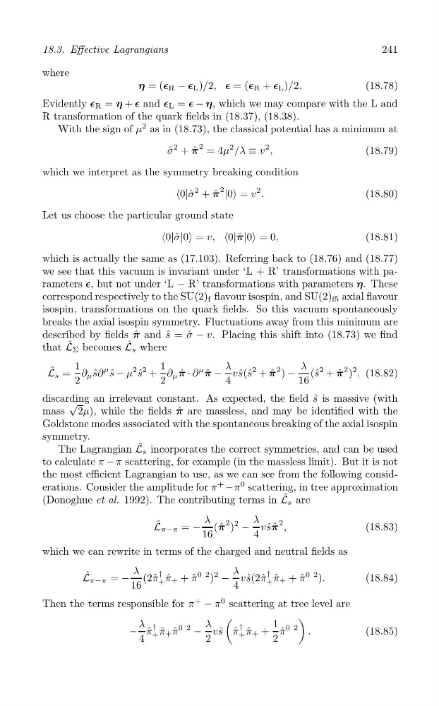
that L ˆ Σ becomes L ˆ s where
1
1
λ
λ
2
2
2
ˆ
∂ μ ˆ s − μ
2 s
L s =
s∂
μ ˆ
ˆ + ∂ μ π ˆ · ∂
μ
π ˆ − vs ˆ(ˆ s + π ˆ
2 ) − (ˆ s + π ˆ
2 )
2 , (18.82)
2
2
4
16
discarding an irrelevant constant. As expected, the field ˆ
s is massive (with
√
mass 2μ), while the fields π ˆ are massless, and may be identified with the
Goldstone modes associated with the spontaneous breaking of the axial isospin
symmetry.
The Lagrangian L ˆ s incorporates the correct symmetries, and can be used
to calculate π − π scattering, for example (in the massless limit). But it is not
the most efficient Lagrangian to use, as we can see from the following considerations. Consider the amplitude for π
+
−π
0 scattering, in tree approximation
(Donoghue et al. 1992). The contributing terms in L ˆ s are
L ˆ π−π = −
λ (π ˆ
2 )
2
−
λ vs ˆπ ˆ
2 ,
(18.83)
16
4
which we can rewrite in terms of the charged and neutral fields as
ˆ
†
π
0 2
†
π
0 2
L π−π = −
λ (2ˆ π π ˆ + + ˆ )
2
−
λ vs ˆ(2ˆ π π ˆ + + ˆ ).
(18.84)
16
+
4
+
Then the terms responsible for π
+
− π
0 scattering at tree level are
(
)
λ
λ
1
†
π
0 2
−
†
π
0 2
− π ˆ π ˆ + ˆ
vs ˆ π ˆ π ˆ + + ˆ
.
(18.85)
4
+
2
+
2